Pediatric Sleep Patterns Detection from Wrist Activity Using Random Forests
Introduction
This research explores the development of a predictive model using wrist-worn accelerometer data to determine a person’s sleep state. Leveraging datasets from the Healthy Brain Network, this study will delve into the nuances of sleep onset and wake events, aiming to revolutionize the understanding of sleep in children.
A total of three data sets will be used in this project, namely train_series.parquet, test_series.parquet, and train_events.csv.
* The Zzzs_train.parquet dataset contains all series to be used as training data. One thing to note is that each series is a continuous recording of accelerometer data for a single subject spanning many days. This dataset has a total of 5 columns, and each column represents an attribute of that accelerometer series. These attributes include series_id - Unique identifier, step - An integer timestep for each observation within a series, timestamp - A corresponding datetime with ISO 8601 format %Y-%m-%dT%H:%M:%S%z, anglez, z-angle is a metric derived from individual accelerometer components that is commonly used in sleep detection, and refers to the angle of the arm relative to the vertical axis of the body, as well as enmo. ENMO is the Euclidean Norm Minus One of all accelerometer signals, with negative values rounded to zero. * The test_series.parquet dataset contains series to be used as the test data, containing the same fields as above. I will predict event occurrences for series in this file. * The train_events.csv file is a complemented dataset that logs specific sleep events such as sleep onset and wake times. This dataset is pivotal in understanding the transitional moments in sleep and serves as a key component in training and refining the predictive models. To be more specific, there are a total of 5 columns, and each column(except the first column, which is just a column of series_id of 12 digits combination of numbers and characters) represents an unique identifier for each series of accelerometer data in Zzzs_train.parquet. These attributes include basic statistics such as night - An enumeration of potential onset / wakeup event pairs. At most one pair of events can occur for each night, and event - The type of event, whether onset or wakeup, as well as step and timestamp, which is the recorded time of occurence of the event in the accelerometer series.
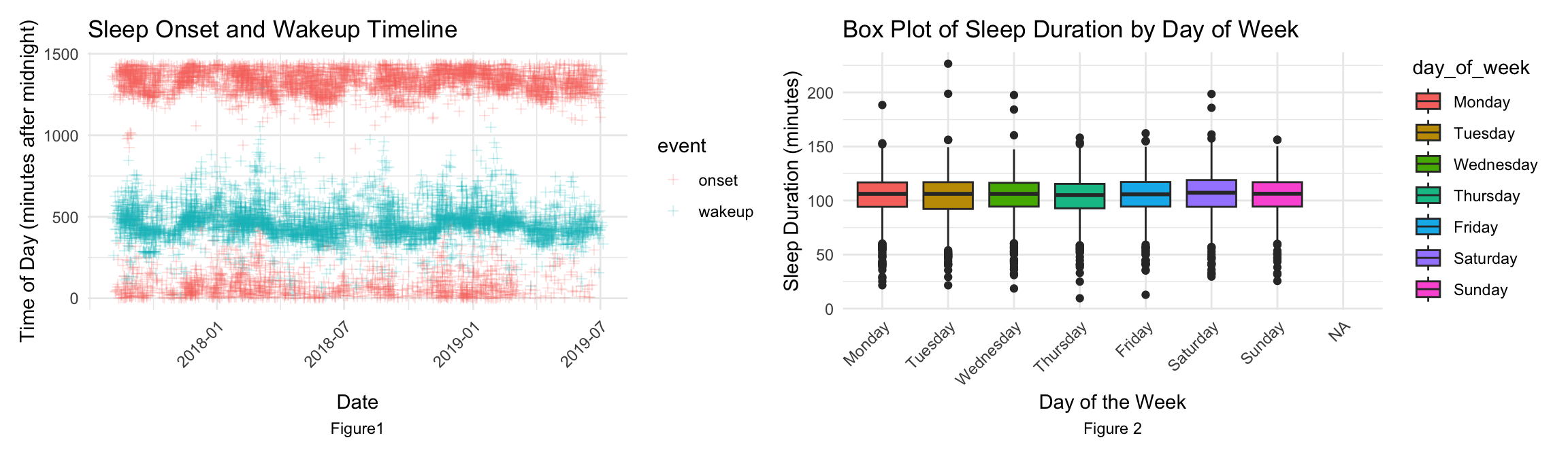
The sleep onset and wakeup timeline plot and the boxplot of sleep duration by day of week motivate the exploration into the sleep patterns. Therefore, central to this research is the question: How can we leverage a machine learning model, trained on wrist-worn accelerometer data, to effectively discern and predict individual sleep patterns and disturbances? Addressing this question can help interpret accelerometer data and have the potential to inform interventions and strategies in child psychology and sleep medicine, offering a new lens through which we can view and understand sleep.
Methodology
Data Preparation & Feature Engineering: The dataset was cleaned thoroughly, prepared for modeling, addressing missing values through deletion. Feature selection was based on the exploratory analysis towards the data distribution patterns, correlation analysis and also the domain knowledge that the wearables position and the sleep hour habits are influential factors to a person’s sleep patterns. Based on these, several key features were extracted from the accelerometer data, including anglez and enmo metrics, which are indicators of the wearer’s movement intensity and orientation, step, event, hour and series_id. These must be crucial factors to be included in the model. Besides, normalization/standardization of data was implemented after exploratory data analysis but before model training to ensure equal contribution of each feature, preventing bias towards variables with larger magnitudes.
From the explortary data analysis on the train_events dataset, the sleep onset and wakeup timeline plot shows as time advanced from late 2017 through to July 2019[Figure1], the observed sleeping patterns exhibit a notable degree of stability and consistency. Predominantly, the awakening time clusters around the 500-minute mark post-midnight, which translates to 8:20 AM. In contrast, the commencement of sleep predominantly spans from 1320 to 1440 minutes after midnight, stretching slightly into the early hours and encapsulating the timeframe from 10:00 PM to 0:30 AM. These findings are in harmonious alignment with conventional sleep schedules typically adhered to, reinforcing their validity within the context of established sleep norms. This detected sleep pattern motivate the model development.
There are some findings from data wrangling as well. Exploring weekly patterns in sleep duration by classifying the data according to each day of the week is also a worthwhile task. The boxplot[Figure2] revealed that sleep durations are generally similar across weekdays and weekends, with two notable exceptions. Saturday showed a marginally longer sleep duration compared to other days, while Thursday emerged as the day with the least amount of sleep. This observation aligns with common expectations, as Thursdays, being mid-week, often involve intensive workloads in anticipation of the weekend, potentially leading to reduced sleep. Conversely, Saturdays provide an opportunity for extended rest and recuperation, especially given the possibility of waking up later on Sunday mornings. However, sleep duration on Sundays does not significantly extend, likely due to the need to wake up early on Mondays. But there’s no much variation among days of week, we can dismiss the day of week factor in our model development.
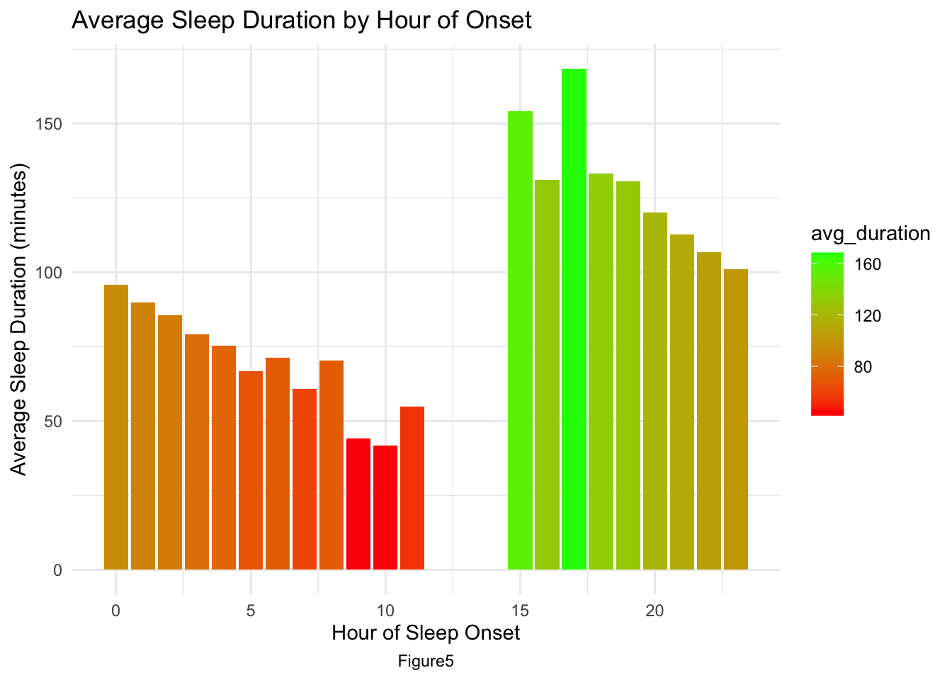
The average sleep duration by hour of onset plot[AppendixB: Figure5] clearly illustrates a distinct trend: as the bedtime shifts to a later hour, there is a corresponding decrease in the total duration of sleep. This pattern suggests that later sleep onset times are often not compensated by equivalent delays in waking up, resulting in shorter overall sleep periods.
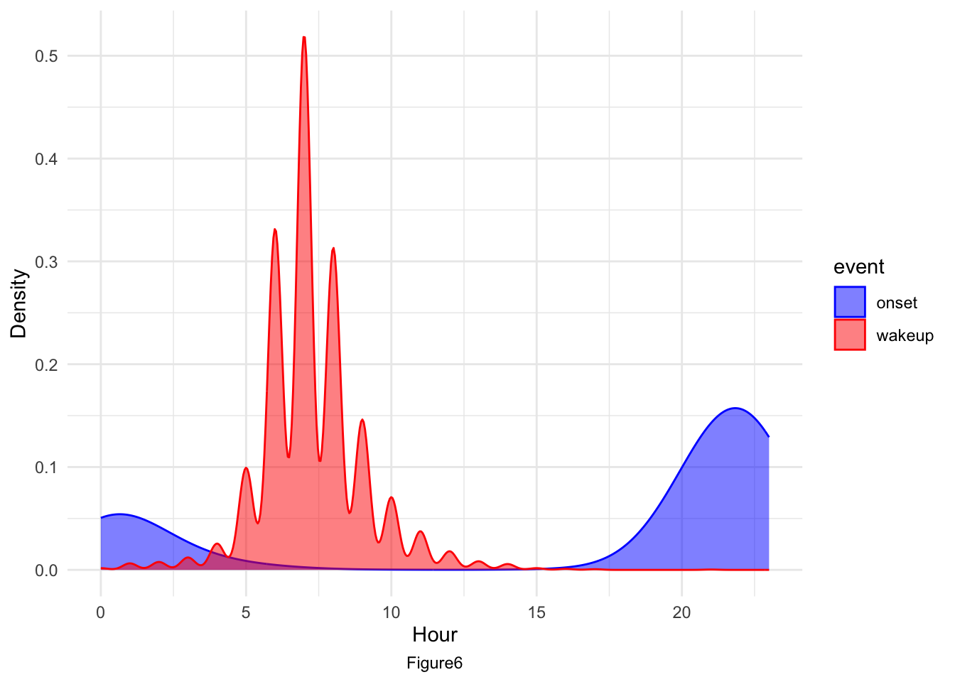
The density plot for sleep onset and wake-up times over time[AppendixB: Figure6] clearly reveals distinct peak periods for each. Wake-up times predominantly peak between 6 to 7 AM, whereas sleep onset times are more broadly distributed, ranging from 10 PM to an hour past midnight. This finding aligns with our previous plots depicting sleep onset and wake-up timelines.
Model Choice: After researching many related literature, the study employs the Random Forest algorithm, selected for its robust performance in complex, high-dimensional classification tasks, and widely used in sleep detection tasks. This choice is preferable over alternatives like logistic regression or support vector machines due to the algorithm’s capability to handle non-linear relationships and provide insights into feature importance, which is crucial for the analysis. I started the codes from scratch in my own way, combing both R and Python tools, implemented a fine-tuned data model, and evaluated in details.
Validation and Testing: The model was trained on the train_series dataset and validated using a subset of the data. The final model was then tested on the test_series dataset to predict sleep states. A confidence score metric quantifying the model’s certainty in its predictions about specific sleep-related events, such as the onset or cessation (wakeup) of sleep was derived from model’s probability predictions. It takes the highest probability from the set of probabilities predicted for each data point, reflecting the model’s most confident prediction.
Results
The model achieves peak accuracy with a small number of predictors. This indicates that a few predictors may be highly informative and sufficient to capture the necessary pattern in the data for accurate predictions. As more predictors are added beyond the optimal point, accuracy declines, which can be indicative of overfitting. The model starts to learn the noise in the training data rather than the underlying pattern. In this case, using 3 predictors might be the optimal complexity for the model.
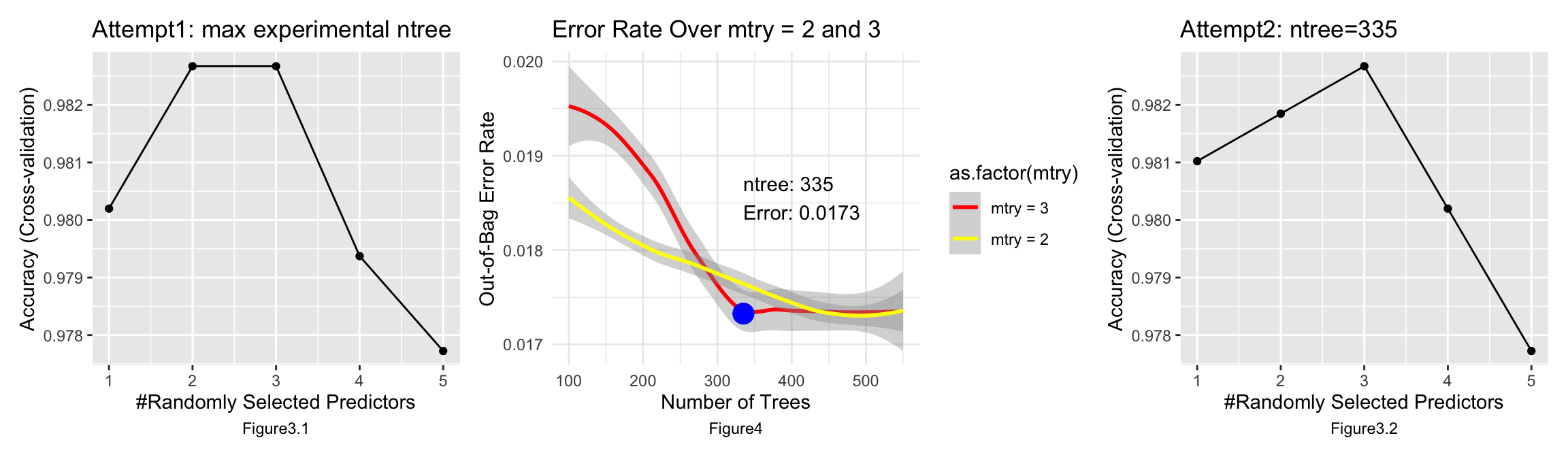
I started training the model with 100 trees and tuning the number of predictors to be sampled between 1 and 5 with 1 as the increment. It turned out that randomly sampling 3 predictors and predicting 335 trees maximized and stabilized the accuracy of model prediction, which is 0.9827, and in this setting, the out-of-bag error rate is 0.0173.
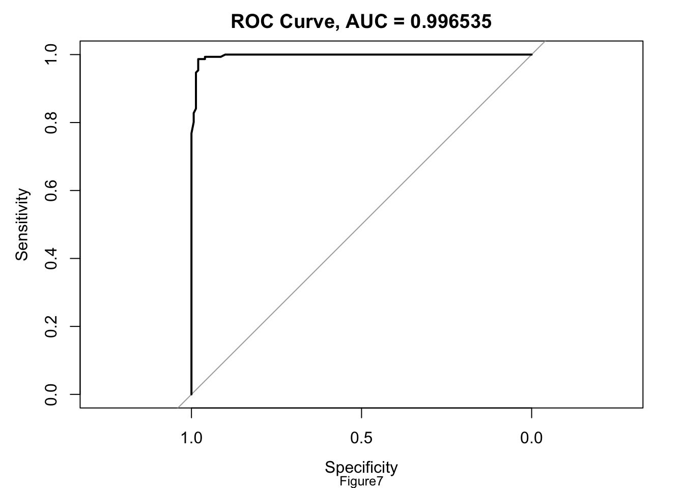
The ROC curve for the model[AppendixB: Figure7] truly looks like a nearly perfect upper triangle, it suggests that the model has near-perfect classification accuracy. This might indicate some form of data leakage or overfitting. So I checked precision, recall, F1 score, and confusion matrices to see whether this might be an imbalanced dataset. However, the accuracy is at 98.34%, Kappa is 0.9669, both recall and specificity are above 98%, precision and negative predictive values are high, balanced accuracy indicating consistent performance, F1 score is at around 0.98. High performance across all these metrics does not suggest a pressing need for sampling methods to address class imbalance.
Lastly, I applied an evaluation metric for event detection in time series and video namely Event Detection Average Precision(EDAP) to the testing set predictions, and got a high sore. Its IOU threshold with tolerance can be replaced. The timestamp error tolerance are custom defined, [12, 36, 60, 90, 120, 150, 180, 240, 300, 360] for onset and same for wakeup event. For each event × tolerance group, the Average Precision (AP) score is calculated, which is the area under the precision-recall curve generated by decreasing confidence score thresholds over the predictions. Multiple AP scores are first averaged over tolerance, then over event to produce a single overall score.
The feature importance plot[AppendixB: Figure8] shows the top3 most influential features were identified as hour of the day, enmo, and anglez, indicating the significance of movement intensity, orientation, and time in determining sleep states. The hour is most influential makes sense since the sleeping patterns are associated with the time hour for sure, and usually a rountine for many people.
The final submission file resembles the example in Appendix C, which is the results tested on a small dataset, where each series has its own onset and wakeup timepoints (indicated by ‘step’) along with a prediction confidence score. The sample results are also consistent with our knowledge, lower confidence score, more likely for a false report. For instance, the indicated potential onset events during noon and afternoon have pretty low confidence score. It is the fact that few people go to bed such early but may get up in the afternoon. One method to determine the confidence score is provided, in addition to this, filtering methods are also experimented in this project, which can be employed to detect only those events where the time gap between onset and wakeup exceeds a certain number of hours (e.g., 6 hours; this threshold can be adjusted based on needs), or by requiring that the confidence score for either onset or wakeup is above 60%. If these criteria are not met, it is likely that no event occurred within the 2.5-hour recording period of that series.
Conclusion
This study successfully demonstrates the potential of using accelerometer data in sleep state detection. Several methods and parameters desgined for the wearables settings are applied, such as the timestamp error tolerance, etc. The high accuracy, AUC scores, event average precision, and recall achieved by the Random Forest model highlight its effectiveness. An exploration into the GGIR package specially for accelerometer data is provided as well, but in this study, even I took methods to transform raw data parquet into csv, the GGIR has very strict requirements for data format. My implementation without using GGIR is more suitable for these datasets. However, a critical limitation of the current model, which employs a random forest algorithm, pertains to its treatment of data. The model operates under the premise that each data point, or timepoint, is an isolated event, devoid of temporal correlation with preceding or subsequent data points. This assumption is a significant departure from the inherently sequential and interdependent nature of sleep patterns. In the realm of sleep studies, where temporal sequences and the continuity of data play pivotal roles, this approach might oversimplify complex biological processes. Therefore, the model may not fully capture the nuanced dynamics of sleep transitions. To enhance the model’s predictive accuracy and clinical relevance, future research should focus on incorporating techniques that recognize and integrate the temporal correlations inherent in sleep patterns. Furthermore, future work could include the application of this model to a broader dataset and exploring other combination techniques (eg. RNN+LSTM) for potential accuracy enhancement. Throughout this research, privacy and data security standards were maintained, and strict adherence to ethical guidelines was ensured to prevent any data misuse, underscoring its sole use in enhancing pediatric healthcare research and practices.
References
Cole, R. J., Kripke, D. F., Gruen, W., Mullaney, D. J., & Gillin, J. C. (1992). Automatic sleep/wake identification from wrist activity. Sleep, 15(5), 461–469. https://doi.org/10.1093/sleep/15.5.461
de Zambotti, M., Cellini, N., Goldstone, A., Colrain, I. M., & Baker, F. C. (2019). Wearable Sleep Technology in Clinical and Research Settings. Medicine and science in sports and exercise, 51(7), 1538–1557. https://doi.org/10.1249/MSS.0000000000001947
Nathalia Esper, Maggie Demkin, Ryan Hoolbrok, Yuki Kotani, Larissa Hunt, Andrew Leroux, Vincent van Hees, Vadim Zipunnikov, Kathleen Merikangas, Michael Milham, Alexandre Franco, Gregory Kiar..(2023). Child Mind Institute - Detect Sleep States. Kaggle. https://kaggle.com/competitions/child-mind-institute-detect-sleep-states
Sundararajan, K., Georgievska, S., Te Lindert, B. H. W., Gehrman, P. R., Ramautar, J., Mazzotti, D. R., Sabia, S., Weedon, M. N., van Someren, E. J. W., Ridder, L., Wang, J., & van Hees, V. T. (2021). Sleep classification from wrist-worn accelerometer data using random forests. Scientific reports, 11(1), 24. https://doi.org/10.1038/s41598-020-79217-x
Appendix
Appendix A: Additional Dataset Details
Detailed Dataset Information
Train Events (train_events.csv)
Accessible through this link, this dataset comprises sleep logs from accelerometer devices, documenting onset and wake events. It contains five columns, including night (enumeration of potential onset/wakeup event pairs), event (type of event), step, and timestamp.
Training Data (Zzzs_train.parquet)
Available here, this dataset includes continuous accelerometer recordings. It features metrics like series_id, step, timestamp, anglez, and enmo, the latter two being crucial metrics for sleep detection as described by the GGIR package.enmo (Euclidean Norm Minus One with negative values rounded to zero) is an acceleration metric describing physical activities. anglez is the angle of the arm relative to the vertical axis of the body.
Test Data (test_series.parquet)
This dataset, used for testing, mirrors the structure of the training data. It can be accessed here.
Appendix B: Additional Plots
Confusion Matrix and Statistics

          Reference
Prediction   0   1
         0 148   2
         1   3 149

               Accuracy : 0.9834
                 95% CI : (0.9618, 0.9946)
    No Information Rate : 0.5
    P-Value [Acc > NIR] : <2e-16

                  Kappa : 0.9669

 Mcnemar's Test P-Value : 1

            Sensitivity : 0.9801
            Specificity : 0.9868
         Pos Pred Value : 0.9867
         Neg Pred Value : 0.9803
             Prevalence : 0.5000
         Detection Rate : 0.4901
   Detection Prevalence : 0.4967
      Balanced Accuracy : 0.9834

       'Positive' Class : 0
[1] "Precision: 0.986666666666667"[1] "Recall: 0.980132450331126"[1] "F1 Score: 0.983388704318937"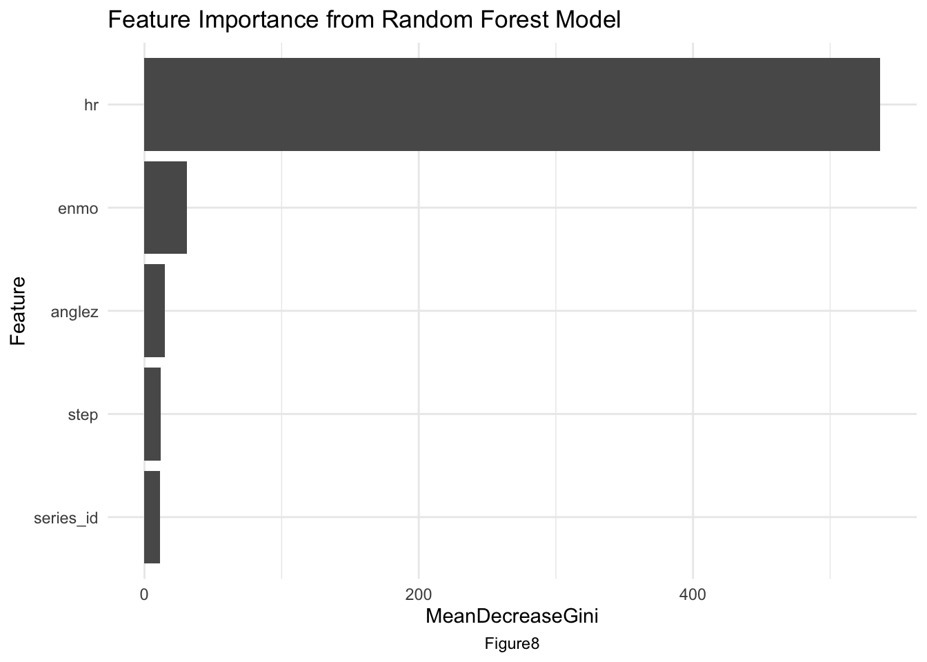
Appendix C: Tests on A Small Sample Data
# A tibble: 8 × 5
  row_id series_id     step event  score
   <dbl> <chr>        <dbl> <chr>  <dbl>
1      0 038441c925bb   124 onset  0.958
2      1 038441c925bb   922 wakeup 0.901
3      2 038491c925aa   315 onset  0.731
4      3 038491c925aa   478 wakeup 0.949
5      4 03d92c9f6f8a   730 onset  0.2
6      5 03d92c9f6f8a   724 wakeup 0.955
7      6 0402a003dae9   842 onset  0.233
8      7 0402a003dae9   839 wakeup 0.949
Appendix D: Code Details
#- Load libraries
library(tidyverse)
library(arrow)
library(skimr)
library(dplyr)
library(ggplot2)
library(lubridate)
library(caret)
library(randomForest)
library(patchwork)
library(pROC)
library(purrr)
#- Read train_events and modify timestamp with lubridate

#- Read events
events <- read_csv("train_events.csv") %>%
        mutate(dt = as_datetime(timestamp)) %>%
        mutate(dt = dt - hours(4))  %>% mutate(hr = hour(dt)) %>%
        select(-timestamp)
head(events)
#- Events counts
events %>% count(event)
#- Sleep onset and wakeup timeline
# Merge onset and wakeup data on dates
timeline_data <- events %>%
  filter(event %in% c("onset", "wakeup")) %>%
  group_by(date = as.Date(dt)) %>%
  mutate(time_minutes = hour(dt) * 60 + minute(dt))

# Create a scatter plot
plot1 <- ggplot(timeline_data, aes(x = date, y = time_minutes, color = event)) +
  geom_point(shape = 3, alpha = 0.2) +
  labs(title = "Sleep Onset and Wakeup Timeline",
       x = "Date",
       y = "Time of Day (minutes after midnight)") +
  theme_minimal() +
  theme(axis.text.x = element_text(angle = 45, hjust = 1))

# Calculate sleep durations and onset hour
pivot_data <- events %>%
  group_by(series_id, night) %>%
  summarize(duration_minutes = (max(step) - min(step)) / 60,
            onset_hour = hour(min(dt)),.groups = 'drop')

# Calculate average sleep duration by hour of onset
average_duration_by_hour <- pivot_data %>%
  group_by(onset_hour) %>%
  summarize(avg_duration = mean(duration_minutes),.groups = 'drop')

# Create a bar plot
plot2 <- ggplot(average_duration_by_hour, aes(x = onset_hour, y = avg_duration, fill = avg_duration)) +
  geom_bar(stat = "identity") +
  labs(title = "Average Sleep Duration by Hour of Onset",
       x = "Hour of Sleep Onset",
       y = "Average Sleep Duration (minutes)") +
  theme_minimal() +
  scale_fill_gradient(low = "red", high = "green")
# Order days of the week
ordered_days <- c("Monday", "Tuesday", "Wednesday", "Thursday", "Friday", "Saturday", "Sunday")
# Extract day of week and calculate sleep duration in minutes
# Calculate sleep duration in minutes and extract day of the week
pivot_data <- events %>%
  group_by(series_id, night) %>%
  summarize(duration_minutes = (max(step) - min(step)) / 60,
            min_datetime = min(dt),.groups = 'drop') %>%
  mutate(day_of_week = factor(format(min_datetime, "%A"), levels = ordered_days))

# Create a box plot
plot3 <- ggplot(pivot_data, aes(x = day_of_week, y = duration_minutes, fill = day_of_week)) +
  geom_boxplot() +
  labs(title = "Box Plot of Sleep Duration by Day of Week",
       x = "Day of the Week",
       y = "Sleep Duration (minutes)") +
  theme_minimal() +
  theme(axis.text.x = element_text(angle = 45, hjust = 1))
#- Distribution of wakeup and Distribution of onset
# Filter the data for "wakeup" and "onset" events
events_wakeup <- events %>% filter(event == "wakeup")
events_onset <- events %>% filter(event == "onset")

# Combine the filtered data into a single data frame
combined_events <- rbind(events_wakeup, events_onset)

# Create the plot with density lines for "wakeup" and "onset" events
plot4 <- ggplot(combined_events, aes(x = hr, color = event, fill = event)) +
  geom_density(alpha = 0.5) +
  labs(x = "Hour", y = "Density") +
  scale_color_manual(values = c("wakeup" = "red", "onset" = "blue")) +
  scale_fill_manual(values = c("wakeup" = "red", "onset" = "blue")) +
  theme_minimal()

# Calculate the number of events per series
events_per_series <- events %>%
  group_by(series_id) %>%
  summarize(num_events = n())

# Create a histogram for the distribution of events per series
plot5 <- ggplot(events_per_series, aes(x = num_events)) +
  geom_histogram(bins = 30, fill = "orange", color = "black", alpha = 0.7) +
  labs(title = "Distribution of Number of Events per Series",
       x = "Number of Events",
       y = "Number of Series") +
  theme_minimal()
# Most series exhibit approximately 48 events. However, there are a few series with a significantly lower number of valid events, which may be excluded from the study.
#- Detect NA in events
events_na <- events %>% group_by(series_id,step) %>% filter(is.na(step))
events_na
num_na <- length(unique(events_na$series_id))
na_id <- unique(events_na$series_id)
num_na
na_id
# Steps containing records with 'NA' (not available) were identified as not precise enough and subsequently removed. Our primary focus was on analyzing accelerometer data that is complete, without any missing values ('NA'). This approach ensures the integrity and reliability of our findings.
#- Series_id without NA events
all_id <- unique(events$series_id)
nna_id <- setdiff(all_id,na_id)
nna_id
# In this study, steps containing records with 'NA' (not available) were identified as not precise enough and subsequently removed. Our primary focus was on analyzing accelerometer data that is complete, without any missing values ('NA'). This approach ensures the integrity and reliability of our findings, as we are utilizing only the most accurate and comprehensive data sets available.
#- Remove two truncated event series
trunc <- c("31011ade7c0a","a596ad0b82aa")
nna_id <- setdiff(nna_id,trunc)
df_nna <- tibble(nna_id) %>% rename(series_id = nna_id)
plot1 <- plot1 + labs(caption = "Figure1")+
                      theme(plot.caption = element_text(hjust = 0.5))
plot3 <- plot3 + labs(caption = "Figure 2")+
                      theme(plot.caption = element_text(hjust = 0.5))

motivate_plot <- plot1 + plot3
                 plot_layout(nrow = 2)

motivate_plot
#- Read training data
train <- read_parquet('Zzzs_train.parquet')
head(train)
nna_train <- right_join(train,df_nna)
nna_event <- right_join(events,df_nna)
train_new <- left_join(nna_train,nna_event)
train_new_full <- right_join(nna_train,nna_event)
head(train_new_full)
training_data <- train_new_full %>%
  select(-timestamp,-event,-dt,-night)
head(training_data)
#- Read testing data
test_old <- read_parquet("test_series.parquet")
# Generate a few random data to enlarge the test_series, the original one only has 3 unique series_id, each series lasts for 2.5 hours.
set.seed(123)
num_rows <- 150
random_data <- data.frame(
  series_id = rep("038441c925bb", num_rows),
  step = 0:(num_rows-1),
  timestamp = seq(from = ymd_hms("2023-12-13T22:30:00-0400"),
                  by = "5 sec", length.out = num_rows),
  anglez = runif(num_rows, min = 0, max = 5),  # Random values between 0 and 5
  enmo = runif(num_rows, min = 0, max = 0.05)  # Random values between 0 and 0.05
)

# Convert timestamps to character
random_data$timestamp <- format(random_data$timestamp, format="%Y-%m-%dT%H:%M:%S-0400")


test <- rbind(test_old, random_data)

random_data <- data.frame(
  series_id = rep("038491c925aa", num_rows),
  step = 0:(num_rows-1),
  timestamp = seq(from = ymd_hms("2020-10-13T23:45:00-0300"),
                  by = "5 sec", length.out = num_rows),
  anglez = runif(num_rows, min = 0, max = 5),  # Random values between 0 and 5
  enmo = runif(num_rows, min = 0, max = 0.05)  # Random values between 0 and 0.05
)

# Convert timestamps to character
random_data$timestamp <- format(random_data$timestamp, format="%Y-%m-%dT%H:%M:%S-0500")

test <- rbind(test, random_data)

random_data <- data.frame(
  series_id = rep("038491c925aa", num_rows),
  step = 0:(num_rows-1),
  timestamp = seq(from = ymd_hms("2021-02-13T02:36:00-0400"),
                  by = "5 sec", length.out = num_rows),
  anglez = runif(num_rows, min = 0, max = 5),  # Random values between 0 and 5
  enmo = runif(num_rows, min = 0, max = 0.05)  # Random values between 0 and 0.05
)

# Convert timestamps to character
random_data$timestamp <- format(random_data$timestamp, format="%Y-%m-%dT%H:%M:%S-0500")

test <- rbind(test, random_data)

test <- test  %>%
        mutate(dt = as_datetime(timestamp)) %>%
        mutate(dt = dt - hours(4)) %>%
        mutate(hr = hour(dt)) %>%
        mutate(step = hr*60+step) %>%
        select(-timestamp,-dt)

head(test)
set.seed(123)
split <- createDataPartition(training_data$awake, p = 0.8, list = FALSE)
training_set <- training_data[split, ]
training_set$awake <- as.factor(training_set$awake)
testing_set <- training_data[-split, ]
testing_set$awake <- as.factor(testing_set$awake)
preprocessing_method <- "standardize"  # or "normalize"
preprocess_params <-  preProcess(training_set, method = ifelse(preprocessing_method == "standardize", c("center", "scale"), c("range")))
saveRDS(preprocess_params, file = "preprocess_params.rds")
preprocessed_training_set <- predict(preprocess_params, training_set)

# Initialize a data frame to store results
results_df <- data.frame(ntree = integer(), mtry = integer(), OOBError = numeric())

# Define the range for mtry and ntree
mtry_range <- seq(1, ncol(preprocessed_training_set) - 1, by=1)  # Full range for predictors
ntree_range <- seq(100, 550, by=5)  # range for ntree

# Loop over mtry and ntree values
for (mtry in mtry_range) {
  for (ntree in ntree_range) {
    set.seed(123)
    model <- randomForest(awake ~ ., data = preprocessed_training_set, mtry = mtry, ntree = ntree, do.trace=FALSE)

    # Extract OOB error rate
    OOBError <- model$err.rate[nrow(model$err.rate), "OOB"]

    # Store results
    results_df <- rbind(results_df, data.frame(ntree = ntree, mtry = mtry, OOBError = OOBError))
  }
}

# Check if results_df is empty or has NA values
if (nrow(results_df) == 0 || any(is.na(results_df$OOBError))) {
  stop("No data to plot. Check the random forest model training.")
}

# Plot accuracy vs. mtry (plot accuracy for different mtry at a fixed ntree)
# Calculate accuracy from the OOB error rate
results_df$Accuracy <- 1 - results_df$OOBError
accuracy_plot <- ggplot(subset(results_df, ntree == 550), aes(x = mtry, y = Accuracy)) +
  geom_line() +
  geom_point() +
  labs(title = "Attempt1: max experimental ntree",
       x = "#Randomly Selected Predictors",
       y = "Accuracy (Cross-validation)")
print(accuracy_plot)
# Filter the results for mtry = 2 and mtry = 3
filtered_df <- results_df[results_df$mtry %in% c(2, 3), ]

# Find local minima for each mtry group
local_minima <- filtered_df %>%
  group_by(mtry) %>%
  slice(which(diff(sign(diff(OOBError))) == 2) + 1) %>%
  ungroup()
specific_minima <- local_minima[5, ]

label_point <- data.frame(
  ntree = 335,
  OOBError = 0.01732673,
  label = "ntree: 335\nError: 0.0173")


# Plot OOB error rates for mtry = 2 and mtry = 3
oob_error_plot <- ggplot(filtered_df, aes(x = ntree, y = OOBError, color = as.factor(mtry), group = mtry)) +
  geom_smooth() +
  geom_point(data = specific_minima, aes(x = ntree, y = OOBError), color = "blue", size = 5, shape = 21, fill = "blue") +
  geom_text(data = label_point, aes(x = ntree, y = OOBError, label = label), nudge_y = 0.001, hjust = 0, vjust = 0, color = "black") +
  xlab("Number of Trees") +
  ylab("Out-of-Bag Error Rate") +
  ggtitle("Error Rate Over mtry = 2 and 3") +
  scale_color_manual(values = c("red", "yellow"), labels = c("mtry = 3", "mtry = 2")) +
  theme_minimal()

print(oob_error_plot)
results_df$Accuracy <- 1 - results_df$OOBError
accuracy_plot2 <- ggplot(subset(results_df, ntree == 335), aes(x = mtry, y = Accuracy)) +
  geom_line() +
  geom_point() +
  labs(title = "Attempt2: ntree=335",
       x = "#Randomly Selected Predictors",
       y = "Accuracy (Cross-validation)")
print(accuracy_plot2)
accuracy_plot <- accuracy_plot+labs(caption = "Figure3.1")+theme(plot.caption = element_text(hjust = 0.5))
oob_error_plot <- oob_error_plot+labs(caption = "Figure4")+theme(plot.caption = element_text(hjust = 0.5))
accuracy_plot2 <- accuracy_plot2+labs(caption = "Figure3.2")+theme(plot.caption = element_text(hjust = 0.5))
hyperparam_plot <- accuracy_plot+oob_error_plot+accuracy_plot2
                 plot_layout(nrow = 2)
hyperparam_plot
preprocessed_training_set$awake <- as.factor(preprocessed_training_set$awake)
model <- randomForest(awake ~ ., data = preprocessed_training_set, ntree = 335, mtry = 3)
saveRDS(model, file = "ReducRFmodel.rds")
# Calculate training accuracy
confusion_matrix <- model$confusion
training_accuracy <- sum(diag(confusion_matrix)) / sum(confusion_matrix)
print(confusion_matrix)
print(paste("Training Accuracy:", training_accuracy))
oob_error <- model$err.rate[nrow(model$err.rate), "OOB"]
training_oob_accuracy <- 1 - oob_error
print(paste("OOB Error Rate:", oob_error))
print(paste("Training OOB Accuracy:", training_oob_accuracy))
preprocess_params <- readRDS(file = "preprocess_params.rds")
# Apply the same preprocessing to the test data
preprocessed_testing_set <- predict(preprocess_params, testing_set)
# Ensure that 'predict' function returns probabilities
testing_set_probs <- predict(model, preprocessed_testing_set, type = "prob")
# Extract probabilities for the positive class ( '1' is the positive class)
positive_class_probs <- testing_set_probs[, "1"]
# Calculate ROC object
roc_obj <- roc(preprocessed_testing_set$awake, positive_class_probs)
# Calculate the AUC
auc_value <- auc(roc_obj)
print(auc_value)
# Plot the ROC curve along with AUC
plot(roc_obj, main=paste("ROC Curve, AUC =", round(auc_value, 6)))
write.csv(testing_set, "testing_set.csv", row.names = FALSE)
write.csv(testing_set_probs, "testing_set_probs.csv", row.names = FALSE)

# Extracting predicted class labels with a threshold. I use 0.5 here
predicted_labels <- ifelse(testing_set_probs[, "1"] > 0.5, 1, 0)

# Confusion Matrix
confusionMatrix <- confusionMatrix(factor(predicted_labels), factor(preprocessed_testing_set$awake))

# Printing the Confusion Matrix
print(confusionMatrix)

# Precision, Recall, and F1 Score
precision <- posPredValue(factor(predicted_labels), factor(preprocessed_testing_set$awake))
recall <- sensitivity(factor(predicted_labels), factor(preprocessed_testing_set$awake))
f1_score <- 2 * ((precision * recall) / (precision + recall))

# Printing the metrics
print(paste("Precision:", precision))
print(paste("Recall:", recall))
print(paste("F1 Score:", f1_score))
# Extract feature importance
importance <- importance(model)
colnames(importance)
feature_importance <- data.frame(
  Feature = rownames(importance),
  Importance = importance[, "MeanDecreaseGini"]
)
# Plot using ggplot2
rf_feature_importance_plot <- ggplot(feature_importance, aes(x = reorder(Feature, Importance), y = Importance)) +
  geom_bar(stat = "identity") +
  coord_flip() +  # Flips the axes for horizontal bars
  xlab("Feature") +
  ylab("MeanDecreaseGini") +
  ggtitle("Feature Importance from Random Forest Model") +
  theme_minimal()
preprocess_params <- readRDS(file = "preprocess_params.rds")
# Apply the same preprocessing to the test data
preprocessed_test <- predict(preprocess_params, test)
# Predict probabilities
# This returns a matrix with probabilities for each class
prob_predictions <- predict(model, newdata = preprocessed_test, type = "prob")

# Determine the predicted class based on the higher probability
# And extract the corresponding confidence score
test$predicted_event <- apply(prob_predictions, 1, function(x) names(x)[which.max(x)])
test$confidence_score <- apply(prob_predictions, 1, max)

# Prepare submission data frame and Write
submission <- test %>%
  select(series_id, step, predicted_event, confidence_score)
write.csv(submission, "submission.csv", row.names = FALSE)
# Predict probabilities
prob_predictions <- predict(model, newdata = preprocessed_test, type = "prob")
# Add predicted probabilities to the test data
test$onset_confidence <- prob_predictions[,"1"]
test$wakeup_confidence <- prob_predictions[,"0"]

# Determine the most likely onset and wakeup for each series_id
# For each series_id, find the step with the highest confidence for onset and wakeup
final_selection <- test %>%
  group_by(series_id) %>%
  summarize(
    onset_step = step[which.max(onset_confidence)],
    onset_score = max(onset_confidence),
    wakeup_step = step[which.max(wakeup_confidence)],
    wakeup_score = max(wakeup_confidence)
  ) %>%
  ungroup()

# Reshape the data for submission
final_submission <- final_selection %>%
  select(series_id, onset_step, onset_score, wakeup_step, wakeup_score) %>%
  pivot_longer(
    cols = c(onset_step, wakeup_step),
    names_to = "event_type",
    values_to = "step"
  ) %>%
  mutate(
    event = ifelse(event_type == "onset_step", "onset", "wakeup"),
    score = ifelse(event_type == "onset_step", onset_score, wakeup_score)
  ) %>%
  select(-event_type, -onset_score, -wakeup_score)

# Assign row_id
final_submission <- final_submission %>%
  mutate(row_id = row_number() - 1) %>%
  select(row_id, everything())

# Extract the mean values used for centering
step_mean <- preprocess_params$mean["step"]

# Write submission file
write.csv(final_submission, "final_submission.csv", row.names = FALSE)
# # Filter function
# # Define feature columns used in the model
# feature_cols <- c("series_id", "step", "anglez", "enmo", "hr")  # Include 'step' and other features
# # Loop over each series ID
# unique_series_ids<-unique(preprocessed_test$series_id)
# for (series_id in unique_series_ids) {
#     series_data <- preprocessed_test %>% filter(series_id == series_id)
#
#     # Predict events
#     preds <- predict(model, newdata = series_data[feature_cols])
#
#     # Detect sleep onsets and wakeups
#     pred_changes <- c(FALSE, diff(preds) != 0)
#     pred_onsets <- series_data$step[preds == 1 & pred_changes]
#     pred_wakeups <- series_data$step[preds == 0 & pred_changes]
#
#     # Filter and score events
#     valid_periods <- which(pred_wakeups - pred_onsets >= 12 * 30)  # Adjust threshold as needed
#     if (length(valid_periods) > 0) {
#         for (i in valid_periods) {
#             onset_step <- pred_onsets[i]
#             wakeup_step <- pred_wakeups[i]
#             score <- mean(series_data$onset_confidence[onset_step:wakeup_step], na.rm = TRUE)
#
#             # Add to final submission
#             final_submission <- rbind(final_submission, data.frame(
#                 series_id = series_id,
#                 onset_step = onset_step,
#                 wakeup_step = wakeup_step,
#                 score = score
#             ))
#         }
#     }
# }
final_submission
library(reticulate)
use_condaenv("env", required = TRUE)
"""Event Detection Average Precision

An average precision metric for event detection in time series and
video.

"""


import numpy as np
import pandas as pd
import pandas.api.types
from typing import Dict, List, Tuple


class ParticipantVisibleError(Exception):
    pass


# Set some placeholders for global parameters
series_id_column_name = None
time_column_name = None
event_column_name = None
score_column_name = None
use_scoring_intervals = None


def score(
        solution: pd.DataFrame,
        submission: pd.DataFrame,
        tolerances: Dict[str, List[float]],
        series_id_column_name: str,
        time_column_name: str,
        event_column_name: str,
        score_column_name: str,
        use_scoring_intervals: bool = False,
) -> float:
    """Event Detection Average Precision, an AUCPR metric for event detection in
    time series and video.

    This metric is similar to IOU-threshold average precision metrics commonly
    used in object detection. For events occuring in time series, we replace the
    IOU threshold with a time tolerance.

    Submissions are evaluated on the average precision of detected events,
    averaged over timestamp error tolerance thresholds, averaged over event
    classes.

    Detections are matched to ground-truth events within error tolerances, with
    ambiguities resolved in order of decreasing confidence.

    Detailed Description
    --------------------
    Evaluation proceeds in four steps:

    1. Selection - (optional) Predictions not within a series' scoring
    intervals are dropped.
    2. Assignment - Predicted events are matched with ground-truth events.
    3. Scoring - Each group of predictions is scored against its corresponding
    group of ground-truth events via Average Precision.
    4. Reduction - The multiple AP scores are averaged to produce a single
    overall score.

    Selection

    With each series there may be a defined set of scoring intervals giving the
    intervals of time over which zero or more ground-truth events might be
    annotated in that series. A prediction will be evaluated only if it falls
    within a scoring interval. These scoring intervals can be chosen to improve
    the fairness of evaluation by, for instance, ignoring edge-cases or
    ambiguous events.

    It is recommended that, if used, scoring intervals be provided for training
    data but not test data.

    Assignment

    For each set of predictions and ground-truths within the same `event x
    tolerance x series_id` group, we match each ground-truth to the
    highest-confidence unmatched prediction occurring within the allowed
    tolerance.

    Some ground-truths may not be matched to a prediction and some predictions
    may not be matched to a ground-truth. They will still be accounted for in
    the scoring, however.

    Scoring

    Collecting the events within each `series_id`, we compute an Average
    Precision score for each `event x tolerance` group. The average precision
    score is the area under the (step-wise) precision-recall curve generated by
    decreasing confidence score thresholds over the predictions. In this
    calculation, matched predictions over the threshold are scored as TP and
    unmatched predictions as FP. Unmatched ground-truths are scored as FN.

    Reduction

    The final score is the average of the above AP scores, first averaged over
    tolerance, then over event.

    Parameters
    ----------
    solution : pd.DataFrame, with columns:

        `series_id_column_name` identifier for each time series

        `time_column_name` the time of occurence for each event as a numeric type

        `event_column_name` class label for each event

        The solution contains the time of occurence of one or more types of
        event within one or more time series. The metric expects the solution to
        contain the same event types as those given in `tolerances`.

        When `use_scoring_intervals == True`, you may include `start` and `end`
        events to delimit intervals within which detections will be scored.
        Detected events (from the user submission) outside of these events will
        be ignored.

    submission : pd.DataFrame, with columns as above and in addition:

        `score_column_name` the predicted confidence score for the detected event

    tolerances : Dict[str, List[float]]

        Maps each event class to a list of timestamp tolerances used
        for matching detections to ground-truth events.

    use_scoring_intervals: bool, default False

        Whether to ignore predicted events outside intervals delimited
        by `'start'` and `'end'` events in the solution. When `False`,
        the solution should not include `'start'` and `'end'` events.
        See the examples for illustration.

    Returns
    -------
    event_detection_ap : float
        The mean average precision of the detected events.

    Examples
    --------
    Detecting `'pass'` events in football:
    >>> column_names = {
    ...     'series_id_column_name': 'video_id',
    ...     'time_column_name': 'time',
    ...     'event_column_name': 'event',
    ...     'score_column_name': 'score',
    ... }
    >>> tolerances = {'pass': [1.0]}
    >>> solution = pd.DataFrame({
    ...     'video_id': ['a', 'a'],
    ...     'event': ['pass', 'pass'],
    ...     'time': [0, 15],
    ... })
    >>> submission = pd.DataFrame({
    ...     'video_id': ['a', 'a', 'a'],
    ...     'event': ['pass', 'pass', 'pass'],
    ...     'score': [1.0, 0.5, 1.0],
    ...     'time': [0, 10, 14.5],
    ... })
    >>> score(solution, submission, tolerances, **column_names)
    1.0

    Increasing the confidence score of the false detection above the true
    detections decreases the AP.
    >>> submission.loc[1, 'score'] = 1.5
    >>> score(solution, submission, tolerances, **column_names)
    0.6666666666666666...

    Likewise, decreasing the confidence score of a true detection below the
    false detection also decreases the AP.
    >>> submission.loc[1, 'score'] = 0.5  # reset
    >>> submission.loc[0, 'score'] = 0.0
    >>> score(solution, submission, tolerances, **column_names)
    0.8333333333333333...

    We average AP scores over tolerances. Previously, the detection at 14.5
    would match, but adding smaller tolerances gives AP scores where it does
    not match. This results in both a FN, since the ground-truth wasn't
    detected, and a FP, since the detected event matches no ground-truth.
    >>> tolerances = {'pass': [0.1, 0.2, 1.0]}
    >>> score(solution, submission, tolerances, **column_names)
    0.3888888888888888...

    We also average over time series and over event classes.
    >>> tolerances = {'pass': [0.5, 1.0], 'challenge': [0.25, 0.50]}
    >>> solution = pd.DataFrame({
    ...     'video_id': ['a', 'a', 'b'],
    ...     'event': ['pass', 'challenge', 'pass'],
    ...     'time': [0, 15, 0],  # restart time for new time series b
    ... })
    >>> submission = pd.DataFrame({
    ...     'video_id': ['a', 'a', 'b'],
    ...     'event': ['pass', 'challenge', 'pass'],
    ...     'score': [1.0, 0.5, 1.0],
    ...     'time': [0, 15, 0],
    ... })
    >>> score(solution, submission, tolerances, **column_names)
    1.0

    By adding scoring intervals to the solution, we may choose to ignore
    detections outside of those intervals.
    >>> tolerances = {'pass': [1.0]}
    >>> solution = pd.DataFrame({
    ...     'video_id': ['a', 'a', 'a', 'a'],
    ...     'event': ['start', 'pass', 'pass', 'end'],
    ...     'time': [0, 10, 20, 30],
    ... })
    >>> submission = pd.DataFrame({
    ...     'video_id': ['a', 'a', 'a'],
    ...     'event': ['pass', 'pass', 'pass'],
    ...     'score': [1.0, 1.0, 1.0],
    ...     'time': [10, 20, 40],
    ... })
    >>> score(solution, submission, tolerances, **column_names, use_scoring_intervals=True)
    1.0

    """
    # Validate metric parameters
    assert len(tolerances) > 0, "Events must have defined tolerances."
    assert set(tolerances.keys()) == set(solution[event_column_name]).difference({'start', 'end'}),\
        (f"Solution column {event_column_name} must contain the same events "
         "as defined in tolerances.")
    assert pd.api.types.is_numeric_dtype(solution[time_column_name]),\
        f"Solution column {time_column_name} must be of numeric type."

    # Validate submission format
    for column_name in [
        series_id_column_name,
        time_column_name,
        event_column_name,
        score_column_name,
    ]:
        if column_name not in submission.columns:
            raise ParticipantVisibleError(f"Submission must have column '{column_name}'.")

    if not pd.api.types.is_numeric_dtype(submission[time_column_name]):
        raise ParticipantVisibleError(
            f"Submission column '{time_column_name}' must be of numeric type."
        )
    if not pd.api.types.is_numeric_dtype(submission[score_column_name]):
        raise ParticipantVisibleError(
            f"Submission column '{score_column_name}' must be of numeric type."
        )

    # Set these globally to avoid passing around a bunch of arguments
    globals()['series_id_column_name'] = series_id_column_name
    globals()['time_column_name'] = time_column_name
    globals()['event_column_name'] = event_column_name
    globals()['score_column_name'] = score_column_name
    globals()['use_scoring_intervals'] = use_scoring_intervals

    return event_detection_ap(solution, submission, tolerances)


def filter_detections(
        detections: pd.DataFrame, intervals: pd.DataFrame
) -> pd.DataFrame:
    """Drop detections not inside a scoring interval."""
    detection_time = detections.loc[:, time_column_name].sort_values().to_numpy()
    intervals = intervals.to_numpy()
    is_scored = np.full_like(detection_time, False, dtype=bool)

    i, j = 0, 0
    while i < len(detection_time) and j < len(intervals):
        time = detection_time[i]
        int_ = intervals[j]

        # If the detection is prior in time to the interval, go to the next detection.
        if time < int_.left:
            i += 1
        # If the detection is inside the interval, keep it and go to the next detection.
        elif time in int_:
            is_scored[i] = True
            i += 1
        # If the detection is later in time, go to the next interval.
        else:
            j += 1

    return detections.loc[is_scored].reset_index(drop=True)


def match_detections(
        tolerance: float, ground_truths: pd.DataFrame, detections: pd.DataFrame
) -> pd.DataFrame:
    """Match detections to ground truth events. Arguments are taken from a common event x tolerance x series_id evaluation group."""
    detections_sorted = detections.sort_values(score_column_name, ascending=False).dropna()
    is_matched = np.full_like(detections_sorted[event_column_name], False, dtype=bool)
    gts_matched = set()
    for i, det in enumerate(detections_sorted.itertuples(index=False)):
        best_error = tolerance
        best_gt = None

        for gt in ground_truths.itertuples(index=False):
            error = abs(getattr(det, time_column_name) - getattr(gt, time_column_name))
            if error < best_error and gt not in gts_matched:
                best_gt = gt
                best_error = error

        if best_gt is not None:
            is_matched[i] = True
            gts_matched.add(best_gt)

    detections_sorted['matched'] = is_matched

    return detections_sorted


def precision_recall_curve(
        matches: np.ndarray, scores: np.ndarray, p: int
) -> Tuple[np.ndarray, np.ndarray, np.ndarray]:
    if len(matches) == 0:
        return [1], [0], []

    # Sort matches by decreasing confidence
    idxs = np.argsort(scores, kind='stable')[::-1]
    scores = scores[idxs]
    matches = matches[idxs]

    distinct_value_indices = np.where(np.diff(scores))[0]
    threshold_idxs = np.r_[distinct_value_indices, matches.size - 1]
    thresholds = scores[threshold_idxs]

    # Matches become TPs and non-matches FPs as confidence threshold decreases
    tps = np.cumsum(matches)[threshold_idxs]
    fps = np.cumsum(~matches)[threshold_idxs]

    precision = tps / (tps + fps)
    precision[np.isnan(precision)] = 0
    recall = tps / p  # total number of ground truths might be different than total number of matches

    # Stop when full recall attained and reverse the outputs so recall is non-increasing.
    last_ind = tps.searchsorted(tps[-1])
    sl = slice(last_ind, None, -1)

    # Final precision is 1 and final recall is 0
    return np.r_[precision[sl], 1], np.r_[recall[sl], 0], thresholds[sl]


def average_precision_score(matches: np.ndarray, scores: np.ndarray, p: int) -> float:
    precision, recall, _ = precision_recall_curve(matches, scores, p)
    # Compute step integral
    return -np.sum(np.diff(recall) * np.array(precision)[:-1])


def event_detection_ap(
        solution: pd.DataFrame,
        submission: pd.DataFrame,
        tolerances: Dict[str, List[float]],
) -> float:

    # Ensure solution and submission are sorted properly
    solution = solution.sort_values([series_id_column_name, time_column_name])
    submission = submission.sort_values([series_id_column_name, time_column_name])

    # Extract scoring intervals.
    if use_scoring_intervals:
        intervals = (
            solution
            .query("event in ['start', 'end']")
            .assign(interval=lambda x: x.groupby([series_id_column_name, event_column_name]).cumcount())
            .pivot(
                index='interval',
                columns=[series_id_column_name, event_column_name],
                values=time_column_name,
            )
            .stack(series_id_column_name)
            .swaplevel()
            .sort_index()
            .loc[:, ['start', 'end']]
            .apply(lambda x: pd.Interval(*x, closed='both'), axis=1)
        )

    # Extract ground-truth events.
    ground_truths = (
        solution
        .query("event not in ['start', 'end']")
        .reset_index(drop=True)
    )

    # Map each event class to its prevalence (needed for recall calculation)
    class_counts = ground_truths.value_counts(event_column_name).to_dict()

    # Create table for detections with a column indicating a match to a ground-truth event
    detections = submission.assign(matched = False)

    # Remove detections outside of scoring intervals
    if use_scoring_intervals:
        detections_filtered = []
        for (det_group, dets), (int_group, ints) in zip(
            detections.groupby(series_id_column_name), intervals.groupby(series_id_column_name)
        ):
            assert det_group == int_group
            detections_filtered.append(filter_detections(dets, ints))
        detections_filtered = pd.concat(detections_filtered, ignore_index=True)
    else:
        detections_filtered = detections

    # Create table of event-class x tolerance x series_id values
    aggregation_keys = pd.DataFrame(
        [(ev, tol, vid)
         for ev in tolerances.keys()
         for tol in tolerances[ev]
         for vid in ground_truths[series_id_column_name].unique()],
        columns=[event_column_name, 'tolerance', series_id_column_name],
    )

    # Create match evaluation groups: event-class x tolerance x series_id
    detections_grouped = (
        aggregation_keys
        .merge(detections_filtered, on=[event_column_name, series_id_column_name], how='left')
        .groupby([event_column_name, 'tolerance', series_id_column_name])
    )
    ground_truths_grouped = (
        aggregation_keys
        .merge(ground_truths, on=[event_column_name, series_id_column_name], how='left')
        .groupby([event_column_name, 'tolerance', series_id_column_name])
    )
    # Match detections to ground truth events by evaluation group
    detections_matched = []
    for key in aggregation_keys.itertuples(index=False):
        dets = detections_grouped.get_group(key)
        gts = ground_truths_grouped.get_group(key)
        detections_matched.append(
            match_detections(dets['tolerance'].iloc[0], gts, dets)
        )
    detections_matched = pd.concat(detections_matched)

    # Compute AP per event x tolerance group
    event_classes = ground_truths[event_column_name].unique()
    ap_table = (
        detections_matched
        .query("event in @event_classes")
        .groupby([event_column_name, 'tolerance']).apply(
            lambda group: average_precision_score(
                group['matched'].to_numpy(),
                group[score_column_name].to_numpy(),
                class_counts[group[event_column_name].iat[0]],
            )
        )
    )
    # Average over tolerances, then over event classes
    mean_ap = ap_table.groupby(event_column_name).mean().sum() / len(event_classes)

    return mean_ap
import numpy as np
import pandas as pd
import matplotlib.pyplot as plt
import polars as pl
import datetime
from tqdm import tqdm

import plotly.express as px
from plotly.subplots import make_subplots
import plotly.graph_objects as go


tolerances = {
    "onset" : [12, 36, 60, 90, 120, 150, 180, 240, 300, 360],
    'wakeup': [12, 36, 60, 90, 120, 150, 180, 240, 300, 360]
}

column_names = {
    'series_id_column_name': 'series_id',
    'time_column_name': 'step',
    'event_column_name': 'event',
    'score_column_name': 'score',
}

#import data
dt_transforms = [
    pl.col('timestamp').str.to_datetime(),
    (pl.col('timestamp').str.to_datetime().dt.year()-2000).cast(pl.UInt8).alias('year'),
    pl.col('timestamp').str.to_datetime().dt.month().cast(pl.UInt8).alias('month'),
    pl.col('timestamp').str.to_datetime().dt.day().cast(pl.UInt8).alias('day'),
    pl.col('timestamp').str.to_datetime().dt.hour().cast(pl.UInt8).alias('hour')
]

data_transforms = [
    pl.col('anglez').cast(pl.Int16), # Casting anglez to 16 bit integer
    (pl.col('enmo')*1000).cast(pl.UInt16), # Convert enmo to 16 bit uint
]

train_series = pl.scan_parquet('train_series.parquet').with_columns(
    dt_transforms + data_transforms
    )

train_events = pl.read_csv('train_events.csv').with_columns(
    dt_transforms
    )

test_series = pl.scan_parquet('test_series.parquet').with_columns(
    dt_transforms + data_transforms
    )

# Getting series ids as a list for convenience
series_ids = train_events['series_id'].unique(maintain_order=True).to_list()

# Removing series with mismatched counts:
onset_counts = train_events.filter(pl.col('event')=='onset').group_by('series_id').count().sort('series_id')['count']
wakeup_counts = train_events.filter(pl.col('event')=='wakeup').group_by('series_id').count().sort('series_id')['count']

counts = pl.DataFrame({'series_id':sorted(series_ids), 'onset_counts':onset_counts, 'wakeup_counts':wakeup_counts})
count_mismatches = counts.filter(counts['onset_counts'] != counts['wakeup_counts'])

train_series = train_series.filter(~pl.col('series_id').is_in(count_mismatches['series_id']))
train_events = train_events.filter(~pl.col('series_id').is_in(count_mismatches['series_id']))

# Updating list of series ids, not including series with no non-null values.
series_ids = train_events.drop_nulls()['series_id'].unique(maintain_order=True).to_list()

# Feature Engineering start from here
features, feature_cols = [pl.col('hour')], ['hour']

for mins in [5, 30, 60*2, 60*8] :
    features += [
        pl.col('enmo').rolling_mean(12 * mins, center=True, min_periods=1).abs().cast(pl.UInt16).alias(f'enmo_{mins}m_mean'),
        pl.col('enmo').rolling_max(12 * mins, center=True, min_periods=1).abs().cast(pl.UInt16).alias(f'enmo_{mins}m_max')
    ]

    feature_cols += [
        f'enmo_{mins}m_mean', f'enmo_{mins}m_max'
    ]

    # Getting first variations
    for var in ['enmo', 'anglez'] :
        features += [
            (pl.col(var).diff().abs().rolling_mean(12 * mins, center=True, min_periods=1)*10).abs().cast(pl.UInt32).alias(f'{var}_1v_{mins}m_mean'),
            (pl.col(var).diff().abs().rolling_max(12 * mins, center=True, min_periods=1)*10).abs().cast(pl.UInt32).alias(f'{var}_1v_{mins}m_max')
        ]

        feature_cols += [
            f'{var}_1v_{mins}m_mean', f'{var}_1v_{mins}m_max'
        ]

id_cols = ['series_id', 'step', 'timestamp']

train_series = train_series.with_columns(
    features
).select(id_cols + feature_cols)

test_series = test_series.with_columns(
    features
).select(id_cols + feature_cols)

# train dataset preparation method
def make_train_dataset(train_data, train_events, drop_nulls=False) :

    series_ids = train_data['series_id'].unique(maintain_order=True).to_list()
    X, y = pl.DataFrame(), pl.DataFrame()
    for idx in tqdm(series_ids) :

        # Normalizing sample features
        sample = train_data.filter(pl.col('series_id')==idx).with_columns(
            [(pl.col(col) / pl.col(col).std()).cast(pl.Float32) for col in feature_cols if col != 'hour']
        )

        events = train_events.filter(pl.col('series_id')==idx)

        if drop_nulls :
            # Removing datapoints on dates where no data was recorded
            sample = sample.filter(
                pl.col('timestamp').dt.date().is_in(events['timestamp'].dt.date())
            )

        X = X.vstack(sample[id_cols + feature_cols])

        onsets = events.filter((pl.col('event') == 'onset') & (pl.col('step') != None))['step'].to_list()
        wakeups = events.filter((pl.col('event') == 'wakeup') & (pl.col('step') != None))['step'].to_list()

        # NOTE: This will break if there are event series without any recorded onsets or wakeups
        y = y.vstack(sample.with_columns(
            sum([(onset <= pl.col('step')) & (pl.col('step') <= wakeup) for onset, wakeup in zip(onsets, wakeups)]).cast(pl.Boolean).alias('asleep')
            ).select('asleep')
            )

    y = y.to_numpy().ravel()

    return X, y


# apply classifier to get event method
def get_events(series, classifier) :
    '''
    Takes a time series and a classifier and returns a formatted submission dataframe.
    '''

    series_ids = series['series_id'].unique(maintain_order=True).to_list()
    events = pl.DataFrame(schema={'series_id':str, 'step':int, 'event':str, 'score':float})

    for idx in tqdm(series_ids) :

        # Collecting sample and normalizing features
        scale_cols = [col for col in feature_cols if (col != 'hour') & (series[col].std() !=0)]
        X = series.filter(pl.col('series_id') == idx).select(id_cols + feature_cols).with_columns(
            [(pl.col(col) / series[col].std()).cast(pl.Float32) for col in scale_cols]
        )

        # Applying classifier to get predictions and scores
        preds, probs = classifier.predict(X[feature_cols]), classifier.predict_proba(X[feature_cols])[:, 1]

        #NOTE: Considered using rolling max to get sleep periods excluding <30 min interruptions, but ended up decreasing performance
        X = X.with_columns(
            pl.lit(preds).cast(pl.Int8).alias('prediction'),
            pl.lit(probs).alias('probability')
                        )

        # Getting predicted onset and wakeup time steps
        pred_onsets = X.filter(X['prediction'].diff() > 0)['step'].to_list()
        pred_wakeups = X.filter(X['prediction'].diff() < 0)['step'].to_list()

        if len(pred_onsets) > 0 :

            # Ensuring all predicted sleep periods begin and end
            if min(pred_wakeups) < min(pred_onsets) :
                pred_wakeups = pred_wakeups[1:]

            if max(pred_onsets) > max(pred_wakeups) :
                pred_onsets = pred_onsets[:-1]

            # Keeping sleep periods longer than 30 minutes
            sleep_periods = [(onset, wakeup) for onset, wakeup in zip(pred_onsets, pred_wakeups) if wakeup - onset >= 12 * 30]

            for onset, wakeup in sleep_periods :
                # Scoring using mean probability over period
                score = X.filter((pl.col('step') >= onset) & (pl.col('step') <= wakeup))['probability'].mean()

                # Adding sleep event to dataframe
                events = events.vstack(pl.DataFrame().with_columns(
                    pl.Series([idx, idx]).alias('series_id'),
                    pl.Series([onset, wakeup]).alias('step'),
                    pl.Series(['onset', 'wakeup']).alias('event'),
                    pl.Series([score, score]).alias('score')
                ))

    # Adding row id column
    events = events.to_pandas().reset_index().rename(columns={'index':'row_id'})

    return events
# extract from R processed testing_set and testing_pred_prob, then use ap score in python to calculate
import pandas as pd
testing_set = pd.read_csv("testing_set.csv")
testing_set_probs = pd.read_csv("testing_set_probs.csv")
series_id_column_name = 'series_id'
time_column_name = 'step'
event_column_name = 'awake'
score_column_name = 'score'

# Create the solution DataFrame
solution = testing_set[[series_id_column_name, time_column_name, event_column_name]]

# Convert predicted probabilities to class labels using a threshold of 0.5
# The probabilities for class "1" are in the second column of testing_set_probs
predicted_labels = (testing_set_probs.iloc[:, 1] > 0.5).astype(int)

# Create the submission DataFrame
submission = testing_set[[series_id_column_name, time_column_name, event_column_name]]
submission['predicted_label'] = predicted_labels  # Add predicted labels
submission['score'] = testing_set_probs.iloc[:, 1] # Add the probabilities as confidence scores

# Handling scoring intervals if use_scoring_intervals is True
use_scoring_intervals = False  # Set to False if not using scoring intervals
if use_scoring_intervals:
    # Example: Assuming 'start_event' and 'end_event' columns in testing_set
    # These columns should represent the intervals for scoring
    solution['start_event'] = testing_set['start_event']
    solution['end_event'] = testing_set['end_event']
    submission['start_event'] = testing_set['start_event']
    submission['end_event'] = testing_set['end_event']

solution = solution.rename(columns={'awake': 'event'})
submission = submission.rename(columns={'awake': 'event'})
solution['event'] = solution['event'].map({0: 'onset', 1: 'wakeup'})
submission['event'] = submission['event'].map({0: 'onset', 1: 'wakeup'})
solution.to_csv('testing_set_solution.csv',index=False)
submission.to_csv('testing_set_submission.csv',index=False)
rf_ap_score = score(solution, submission, tolerances, **column_names)
plot2+ labs(caption = "Figure5")+
                      theme(plot.caption = element_text(hjust = 0.5))
plot4+ labs(caption = "Figure6")+
                      theme(plot.caption = element_text(hjust = 0.5))
plot(roc_obj, main=paste("ROC Curve, AUC =", round(auc_value, 6)))
mtext("Figure7", side = 1, line = 4.15, cex = 0.8)
# Printing the Confusion Matrix
print(confusionMatrix)
# Printing the metrics
print(paste("Precision:", precision))
print(paste("Recall:", recall))
print(paste("F1 Score:", f1_score))
rf_feature_importance_plot+ labs(caption = "Figure8")+
                      theme(plot.caption = element_text(hjust = 0.5))
final_submission
### An Optional Dive into GGIR Package
train_events <- read.csv("train_events.csv")
train_series <- arrow::read_parquet("Zzzs_train.parquet")
test_series <- arrow::read_parquet("test_series.parquet")
write.csv(train_series, "Zzzs_train.csv", row.names = FALSE)
write.csv(test_series,'test_series.csv', row.names = FALSE)

library(GGIR)
#g.shell.GGIR
#- Load libraries
library(tidyverse)
library(arrow)
library(skimr)
library(dplyr)
library(ggplot2)
library(lubridate)
library(caret)
library(randomForest)
library(patchwork)
library(pROC)
library(purrr)
#- Read train_events and modify timestamp with lubridate
#- Read events
events <- read_csv("train_events.csv") %>%
mutate(dt = as_datetime(timestamp)) %>%
mutate(dt = dt - hours(4)) %>% mutate(hr = hour(dt)) %>%
select(-timestamp)
head(events)
#- Events counts
events %>% count(event)
#- Sleep onset and wakeup timeline
# Merge onset and wakeup data on dates
timeline_data <- events %>%
filter(event %in% c("onset", "wakeup")) %>%
group_by(date = as.Date(dt)) %>%
mutate(time_minutes = hour(dt) * 60 + minute(dt))
# Create a scatter plot
plot1 <- ggplot(timeline_data, aes(x = date, y = time_minutes, color = event)) +
geom_point(shape = 3, alpha = 0.2) +
labs(title = "Sleep Onset and Wakeup Timeline",
x = "Date",
y = "Time of Day (minutes after midnight)") +
theme_minimal() +
theme(axis.text.x = element_text(angle = 45, hjust = 1))
# Calculate sleep durations and onset hour
pivot_data <- events %>%
group_by(series_id, night) %>%
summarize(duration_minutes = (max(step) - min(step)) / 60,
onset_hour = hour(min(dt)),.groups = 'drop')
# Calculate average sleep duration by hour of onset
average_duration_by_hour <- pivot_data %>%
group_by(onset_hour) %>%
summarize(avg_duration = mean(duration_minutes),.groups = 'drop')
# Create a bar plot
plot2 <- ggplot(average_duration_by_hour, aes(x = onset_hour, y = avg_duration, fill = avg_duration)) +
geom_bar(stat = "identity") +
labs(title = "Average Sleep Duration by Hour of Onset",
x = "Hour of Sleep Onset",
y = "Average Sleep Duration (minutes)") +
theme_minimal() +
scale_fill_gradient(low = "red", high = "green")
# Order days of the week
ordered_days <- c("Monday", "Tuesday", "Wednesday", "Thursday", "Friday", "Saturday", "Sunday")
# Extract day of week and calculate sleep duration in minutes
# Calculate sleep duration in minutes and extract day of the week
pivot_data <- events %>%
group_by(series_id, night) %>%
summarize(duration_minutes = (max(step) - min(step)) / 60,
min_datetime = min(dt),.groups = 'drop') %>%
mutate(day_of_week = factor(format(min_datetime, "%A"), levels = ordered_days))
# Create a box plot
plot3 <- ggplot(pivot_data, aes(x = day_of_week, y = duration_minutes, fill = day_of_week)) +
geom_boxplot() +
labs(title = "Box Plot of Sleep Duration by Day of Week",
x = "Day of the Week",
y = "Sleep Duration (minutes)") +
theme_minimal() +
theme(axis.text.x = element_text(angle = 45, hjust = 1))
#- Distribution of wakeup and Distribution of onset
# Filter the data for "wakeup" and "onset" events
events_wakeup <- events %>% filter(event == "wakeup")
events_onset <- events %>% filter(event == "onset")
# Combine the filtered data into a single data frame
combined_events <- rbind(events_wakeup, events_onset)
# Create the plot with density lines for "wakeup" and "onset" events
plot4 <- ggplot(combined_events, aes(x = hr, color = event, fill = event)) +
geom_density(alpha = 0.5) +
labs(x = "Hour", y = "Density") +
scale_color_manual(values = c("wakeup" = "red", "onset" = "blue")) +
scale_fill_manual(values = c("wakeup" = "red", "onset" = "blue")) +
theme_minimal()
# Calculate the number of events per series
events_per_series <- events %>%
group_by(series_id) %>%
summarize(num_events = n())
# Create a histogram for the distribution of events per series
plot5 <- ggplot(events_per_series, aes(x = num_events)) +
geom_histogram(bins = 30, fill = "orange", color = "black", alpha = 0.7) +
labs(title = "Distribution of Number of Events per Series",
x = "Number of Events",
y = "Number of Series") +
theme_minimal()
# Most series exhibit approximately 48 events. However, there are a few series with a significantly lower number of valid events, which may be excluded from the study.
#- Detect NA in events
events_na <- events %>% group_by(series_id,step) %>% filter(is.na(step))
events_na
num_na <- length(unique(events_na$series_id))
na_id <- unique(events_na$series_id)
num_na
na_id
# Steps containing records with 'NA' (not available) were identified as not precise enough and subsequently removed. Our primary focus was on analyzing accelerometer data that is complete, without any missing values ('NA'). This approach ensures the integrity and reliability of our findings.
#- Series_id without NA events
all_id <- unique(events$series_id)
nna_id <- setdiff(all_id,na_id)
nna_id
# In this study, steps containing records with 'NA' (not available) were identified as not precise enough and subsequently removed. Our primary focus was on analyzing accelerometer data that is complete, without any missing values ('NA'). This approach ensures the integrity and reliability of our findings, as we are utilizing only the most accurate and comprehensive data sets available.
#- Remove two truncated event series
trunc <- c("31011ade7c0a","a596ad0b82aa")
nna_id <- setdiff(nna_id,trunc)
df_nna <- tibble(nna_id) %>% rename(series_id = nna_id)
plot1 <- plot1 + labs(caption = "Figure1")+
theme(plot.caption = element_text(hjust = 0.5))
plot3 <- plot3 + labs(caption = "Figure 2")+
theme(plot.caption = element_text(hjust = 0.5))
motivate_plot <- plot1 + plot3
plot_layout(nrow = 2)
motivate_plot
#- Read training data
train <- read_parquet('Zzzs_train.parquet')
head(train)
nna_train <- right_join(train,df_nna)
nna_event <- right_join(events,df_nna)
train_new <- left_join(nna_train,nna_event)
train_new_full <- right_join(nna_train,nna_event)
head(train_new_full)
training_data <- train_new_full %>%
select(-timestamp,-event,-dt,-night)
head(training_data)
#- Read testing data
test_old <- read_parquet("test_series.parquet")
# Generate a few random data to enlarge the test_series, the original one only has 3 unique series_id, each series lasts for 2.5 hours.
set.seed(123)
num_rows <- 150
random_data <- data.frame(
series_id = rep("038441c925bb", num_rows),
step = 0:(num_rows-1),
timestamp = seq(from = ymd_hms("2023-12-13T22:30:00-0400"),
by = "5 sec", length.out = num_rows),
anglez = runif(num_rows, min = 0, max = 5), # Random values between 0 and 5
enmo = runif(num_rows, min = 0, max = 0.05) # Random values between 0 and 0.05
)
# Convert timestamps to character
random_data$timestamp <- format(random_data$timestamp, format="%Y-%m-%dT%H:%M:%S-0400")
test <- rbind(test_old, random_data)
random_data <- data.frame(
series_id = rep("038491c925aa", num_rows),
step = 0:(num_rows-1),
timestamp = seq(from = ymd_hms("2020-10-13T23:45:00-0300"),
by = "5 sec", length.out = num_rows),
anglez = runif(num_rows, min = 0, max = 5), # Random values between 0 and 5
enmo = runif(num_rows, min = 0, max = 0.05) # Random values between 0 and 0.05
)
# Convert timestamps to character
random_data$timestamp <- format(random_data$timestamp, format="%Y-%m-%dT%H:%M:%S-0500")
test <- rbind(test, random_data)
random_data <- data.frame(
series_id = rep("038491c925aa", num_rows),
step = 0:(num_rows-1),
timestamp = seq(from = ymd_hms("2021-02-13T02:36:00-0400"),
by = "5 sec", length.out = num_rows),
anglez = runif(num_rows, min = 0, max = 5), # Random values between 0 and 5
enmo = runif(num_rows, min = 0, max = 0.05) # Random values between 0 and 0.05
)
# Convert timestamps to character
random_data$timestamp <- format(random_data$timestamp, format="%Y-%m-%dT%H:%M:%S-0500")
test <- rbind(test, random_data)
test <- test %>%
mutate(dt = as_datetime(timestamp)) %>%
mutate(dt = dt - hours(4)) %>%
mutate(hr = hour(dt)) %>%
mutate(step = hr*60+step) %>%
select(-timestamp,-dt)
head(test)
set.seed(123)
split <- createDataPartition(training_data$awake, p = 0.8, list = FALSE)
training_set <- training_data[split, ]
training_set$awake <- as.factor(training_set$awake)
testing_set <- training_data[-split, ]
testing_set$awake <- as.factor(testing_set$awake)
preprocessing_method <- "standardize" # or "normalize"
preprocess_params <- preProcess(training_set, method = ifelse(preprocessing_method == "standardize", c("center", "scale"), c("range")))
saveRDS(preprocess_params, file = "preprocess_params.rds")
preprocessed_training_set <- predict(preprocess_params, training_set)
# Initialize a data frame to store results
results_df <- data.frame(ntree = integer(), mtry = integer(), OOBError = numeric())
# Define the range for mtry and ntree
mtry_range <- seq(1, ncol(preprocessed_training_set) - 1, by=1) # Full range for predictors
ntree_range <- seq(100, 550, by=5) # range for ntree
# Loop over mtry and ntree values
for (mtry in mtry_range) {
for (ntree in ntree_range) {
set.seed(123)
model <- randomForest(awake ~ ., data = preprocessed_training_set, mtry = mtry, ntree = ntree, do.trace=FALSE)
# Extract OOB error rate
OOBError <- model$err.rate[nrow(model$err.rate), "OOB"]
# Store results
results_df <- rbind(results_df, data.frame(ntree = ntree, mtry = mtry, OOBError = OOBError))
}
}
# Check if results_df is empty or has NA values
if (nrow(results_df) == 0 || any(is.na(results_df$OOBError))) {
stop("No data to plot. Check the random forest model training.")
}
# Plot accuracy vs. mtry (plot accuracy for different mtry at a fixed ntree)
# Calculate accuracy from the OOB error rate
results_df$Accuracy <- 1 - results_df$OOBError
accuracy_plot <- ggplot(subset(results_df, ntree == 550), aes(x = mtry, y = Accuracy)) +
geom_line() +
geom_point() +
labs(title = "Attempt1: max experimental ntree",
x = "#Randomly Selected Predictors",
y = "Accuracy (Cross-validation)")
print(accuracy_plot)
# Filter the results for mtry = 2 and mtry = 3
filtered_df <- results_df[results_df$mtry %in% c(2, 3), ]
# Find local minima for each mtry group
local_minima <- filtered_df %>%
group_by(mtry) %>%
slice(which(diff(sign(diff(OOBError))) == 2) + 1) %>%
ungroup()
specific_minima <- local_minima[5, ]
label_point <- data.frame(
ntree = 335,
OOBError = 0.01732673,
label = "ntree: 335\nError: 0.0173")
# Plot OOB error rates for mtry = 2 and mtry = 3
oob_error_plot <- ggplot(filtered_df, aes(x = ntree, y = OOBError, color = as.factor(mtry), group = mtry)) +
geom_smooth() +
geom_point(data = specific_minima, aes(x = ntree, y = OOBError), color = "blue", size = 5, shape = 21, fill = "blue") +
geom_text(data = label_point, aes(x = ntree, y = OOBError, label = label), nudge_y = 0.001, hjust = 0, vjust = 0, color = "black") +
xlab("Number of Trees") +
ylab("Out-of-Bag Error Rate") +
ggtitle("Error Rate Over mtry = 2 and 3") +
scale_color_manual(values = c("red", "yellow"), labels = c("mtry = 3", "mtry = 2")) +
theme_minimal()
print(oob_error_plot)
results_df$Accuracy <- 1 - results_df$OOBError
accuracy_plot2 <- ggplot(subset(results_df, ntree == 335), aes(x = mtry, y = Accuracy)) +
geom_line() +
geom_point() +
labs(title = "Attempt2: ntree=335",
x = "#Randomly Selected Predictors",
y = "Accuracy (Cross-validation)")
print(accuracy_plot2)
accuracy_plot <- accuracy_plot+labs(caption = "Figure3.1")+theme(plot.caption = element_text(hjust = 0.5))
oob_error_plot <- oob_error_plot+labs(caption = "Figure4")+theme(plot.caption = element_text(hjust = 0.5))
accuracy_plot2 <- accuracy_plot2+labs(caption = "Figure3.2")+theme(plot.caption = element_text(hjust = 0.5))
hyperparam_plot <- accuracy_plot+oob_error_plot+accuracy_plot2
plot_layout(nrow = 2)
hyperparam_plot
preprocessed_training_set$awake <- as.factor(preprocessed_training_set$awake)
model <- randomForest(awake ~ ., data = preprocessed_training_set, ntree = 335, mtry = 3)
saveRDS(model, file = "ReducRFmodel.rds")
# Calculate training accuracy
confusion_matrix <- model$confusion
training_accuracy <- sum(diag(confusion_matrix)) / sum(confusion_matrix)
print(confusion_matrix)
print(paste("Training Accuracy:", training_accuracy))
oob_error <- model$err.rate[nrow(model$err.rate), "OOB"]
training_oob_accuracy <- 1 - oob_error
print(paste("OOB Error Rate:", oob_error))
print(paste("Training OOB Accuracy:", training_oob_accuracy))
preprocess_params <- readRDS(file = "preprocess_params.rds")
# Apply the same preprocessing to the test data
preprocessed_testing_set <- predict(preprocess_params, testing_set)
# Ensure that 'predict' function returns probabilities
testing_set_probs <- predict(model, preprocessed_testing_set, type = "prob")
# Extract probabilities for the positive class ( '1' is the positive class)
positive_class_probs <- testing_set_probs[, "1"]
# Calculate ROC object
roc_obj <- roc(preprocessed_testing_set$awake, positive_class_probs)
# Calculate the AUC
auc_value <- auc(roc_obj)
print(auc_value)
# Plot the ROC curve along with AUC
plot(roc_obj, main=paste("ROC Curve, AUC =", round(auc_value, 6)))
write.csv(testing_set, "testing_set.csv", row.names = FALSE)
write.csv(testing_set_probs, "testing_set_probs.csv", row.names = FALSE)
# Extracting predicted class labels with a threshold. I use 0.5 here
predicted_labels <- ifelse(testing_set_probs[, "1"] > 0.5, 1, 0)
# Confusion Matrix
confusionMatrix <- confusionMatrix(factor(predicted_labels), factor(preprocessed_testing_set$awake))
# Printing the Confusion Matrix
print(confusionMatrix)
# Precision, Recall, and F1 Score
precision <- posPredValue(factor(predicted_labels), factor(preprocessed_testing_set$awake))
recall <- sensitivity(factor(predicted_labels), factor(preprocessed_testing_set$awake))
f1_score <- 2 * ((precision * recall) / (precision + recall))
# Printing the metrics
print(paste("Precision:", precision))
print(paste("Recall:", recall))
print(paste("F1 Score:", f1_score))
# Extract feature importance
importance <- importance(model)
colnames(importance)
feature_importance <- data.frame(
Feature = rownames(importance),
Importance = importance[, "MeanDecreaseGini"]
)
# Plot using ggplot2
rf_feature_importance_plot <- ggplot(feature_importance, aes(x = reorder(Feature, Importance), y = Importance)) +
geom_bar(stat = "identity") +
coord_flip() + # Flips the axes for horizontal bars
xlab("Feature") +
ylab("MeanDecreaseGini") +
ggtitle("Feature Importance from Random Forest Model") +
theme_minimal()
preprocess_params <- readRDS(file = "preprocess_params.rds")
# Apply the same preprocessing to the test data
preprocessed_test <- predict(preprocess_params, test)
# Predict probabilities
# This returns a matrix with probabilities for each class
prob_predictions <- predict(model, newdata = preprocessed_test, type = "prob")
# Determine the predicted class based on the higher probability
# And extract the corresponding confidence score
test$predicted_event <- apply(prob_predictions, 1, function(x) names(x)[which.max(x)])
test$confidence_score <- apply(prob_predictions, 1, max)
# Prepare submission data frame and Write
submission <- test %>%
select(series_id, step, predicted_event, confidence_score)
write.csv(submission, "submission.csv", row.names = FALSE)
# Predict probabilities
prob_predictions <- predict(model, newdata = preprocessed_test, type = "prob")
# Add predicted probabilities to the test data
test$onset_confidence <- prob_predictions[,"1"]
test$wakeup_confidence <- prob_predictions[,"0"]
# Determine the most likely onset and wakeup for each series_id
# For each series_id, find the step with the highest confidence for onset and wakeup
final_selection <- test %>%
group_by(series_id) %>%
summarize(
onset_step = step[which.max(onset_confidence)],
onset_score = max(onset_confidence),
wakeup_step = step[which.max(wakeup_confidence)],
wakeup_score = max(wakeup_confidence)
) %>%
ungroup()
# Reshape the data for submission
final_submission <- final_selection %>%
select(series_id, onset_step, onset_score, wakeup_step, wakeup_score) %>%
pivot_longer(
cols = c(onset_step, wakeup_step),
names_to = "event_type",
values_to = "step"
) %>%
mutate(
event = ifelse(event_type == "onset_step", "onset", "wakeup"),
score = ifelse(event_type == "onset_step", onset_score, wakeup_score)
) %>%
select(-event_type, -onset_score, -wakeup_score)
# Assign row_id
final_submission <- final_submission %>%
mutate(row_id = row_number() - 1) %>%
select(row_id, everything())
# Extract the mean values used for centering
step_mean <- preprocess_params$mean["step"]
# Write submission file
write.csv(final_submission, "final_submission.csv", row.names = FALSE)
# # Filter function
# # Define feature columns used in the model
# feature_cols <- c("series_id", "step", "anglez", "enmo", "hr") # Include 'step' and other features
# # Loop over each series ID
# unique_series_ids<-unique(preprocessed_test$series_id)
# for (series_id in unique_series_ids) {
# series_data <- preprocessed_test %>% filter(series_id == series_id)
#
# # Predict events
# preds <- predict(model, newdata = series_data[feature_cols])
#
# # Detect sleep onsets and wakeups
# pred_changes <- c(FALSE, diff(preds) != 0)
# pred_onsets <- series_data$step[preds == 1 & pred_changes]
# pred_wakeups <- series_data$step[preds == 0 & pred_changes]
#
# # Filter and score events
# valid_periods <- which(pred_wakeups - pred_onsets >= 12 * 30) # Adjust threshold as needed
# if (length(valid_periods) > 0) {
# for (i in valid_periods) {
# onset_step <- pred_onsets[i]
# wakeup_step <- pred_wakeups[i]
# score <- mean(series_data$onset_confidence[onset_step:wakeup_step], na.rm = TRUE)
#
# # Add to final submission
# final_submission <- rbind(final_submission, data.frame(
# series_id = series_id,
# onset_step = onset_step,
# wakeup_step = wakeup_step,
# score = score
# ))
# }
# }
# }
final_submission
library(reticulate)
use_condaenv("env", required = TRUE)
"""Event Detection Average Precision
An average precision metric for event detection in time series and
video.
"""
import numpy as np
import pandas as pd
import pandas.api.types
from typing import Dict, List, Tuple
class ParticipantVisibleError(Exception):
pass
# Set some placeholders for global parameters
series_id_column_name = None
time_column_name = None
event_column_name = None
score_column_name = None
use_scoring_intervals = None
def score(
solution: pd.DataFrame,
submission: pd.DataFrame,
tolerances: Dict[str, List[float]],
series_id_column_name: str,
time_column_name: str,
event_column_name: str,
score_column_name: str,
use_scoring_intervals: bool = False,
) -> float:
"""Event Detection Average Precision, an AUCPR metric for event detection in
time series and video.
This metric is similar to IOU-threshold average precision metrics commonly
used in object detection. For events occuring in time series, we replace the
IOU threshold with a time tolerance.
Submissions are evaluated on the average precision of detected events,
averaged over timestamp error tolerance thresholds, averaged over event
classes.
Detections are matched to ground-truth events within error tolerances, with
ambiguities resolved in order of decreasing confidence.
Detailed Description
--------------------
Evaluation proceeds in four steps:
1. Selection - (optional) Predictions not within a series' scoring
intervals are dropped.
2. Assignment - Predicted events are matched with ground-truth events.
3. Scoring - Each group of predictions is scored against its corresponding
group of ground-truth events via Average Precision.
4. Reduction - The multiple AP scores are averaged to produce a single
overall score.
Selection
With each series there may be a defined set of scoring intervals giving the
intervals of time over which zero or more ground-truth events might be
annotated in that series. A prediction will be evaluated only if it falls
within a scoring interval. These scoring intervals can be chosen to improve
the fairness of evaluation by, for instance, ignoring edge-cases or
ambiguous events.
It is recommended that, if used, scoring intervals be provided for training
data but not test data.
Assignment
For each set of predictions and ground-truths within the same `event x
tolerance x series_id` group, we match each ground-truth to the
highest-confidence unmatched prediction occurring within the allowed
tolerance.
Some ground-truths may not be matched to a prediction and some predictions
may not be matched to a ground-truth. They will still be accounted for in
the scoring, however.
Scoring
Collecting the events within each `series_id`, we compute an Average
Precision score for each `event x tolerance` group. The average precision
score is the area under the (step-wise) precision-recall curve generated by
decreasing confidence score thresholds over the predictions. In this
calculation, matched predictions over the threshold are scored as TP and
unmatched predictions as FP. Unmatched ground-truths are scored as FN.
Reduction
The final score is the average of the above AP scores, first averaged over
tolerance, then over event.
Parameters
----------
solution : pd.DataFrame, with columns:
`series_id_column_name` identifier for each time series
`time_column_name` the time of occurence for each event as a numeric type
`event_column_name` class label for each event
The solution contains the time of occurence of one or more types of
event within one or more time series. The metric expects the solution to
contain the same event types as those given in `tolerances`.
When `use_scoring_intervals == True`, you may include `start` and `end`
events to delimit intervals within which detections will be scored.
Detected events (from the user submission) outside of these events will
be ignored.
submission : pd.DataFrame, with columns as above and in addition:
`score_column_name` the predicted confidence score for the detected event
tolerances : Dict[str, List[float]]
Maps each event class to a list of timestamp tolerances used
for matching detections to ground-truth events.
use_scoring_intervals: bool, default False
Whether to ignore predicted events outside intervals delimited
by `'start'` and `'end'` events in the solution. When `False`,
the solution should not include `'start'` and `'end'` events.
See the examples for illustration.
Returns
-------
event_detection_ap : float
The mean average precision of the detected events.
Examples
--------
Detecting `'pass'` events in football:
>>> column_names = {
... 'series_id_column_name': 'video_id',
... 'time_column_name': 'time',
... 'event_column_name': 'event',
... 'score_column_name': 'score',
... }
>>> tolerances = {'pass': [1.0]}
>>> solution = pd.DataFrame({
... 'video_id': ['a', 'a'],
... 'event': ['pass', 'pass'],
... 'time': [0, 15],
... })
>>> submission = pd.DataFrame({
... 'video_id': ['a', 'a', 'a'],
... 'event': ['pass', 'pass', 'pass'],
... 'score': [1.0, 0.5, 1.0],
... 'time': [0, 10, 14.5],
... })
>>> score(solution, submission, tolerances, **column_names)
1.0
Increasing the confidence score of the false detection above the true
detections decreases the AP.
>>> submission.loc[1, 'score'] = 1.5
>>> score(solution, submission, tolerances, **column_names)
0.6666666666666666...
Likewise, decreasing the confidence score of a true detection below the
false detection also decreases the AP.
>>> submission.loc[1, 'score'] = 0.5 # reset
>>> submission.loc[0, 'score'] = 0.0
>>> score(solution, submission, tolerances, **column_names)
0.8333333333333333...
We average AP scores over tolerances. Previously, the detection at 14.5
would match, but adding smaller tolerances gives AP scores where it does
not match. This results in both a FN, since the ground-truth wasn't
detected, and a FP, since the detected event matches no ground-truth.
>>> tolerances = {'pass': [0.1, 0.2, 1.0]}
>>> score(solution, submission, tolerances, **column_names)
0.3888888888888888...
We also average over time series and over event classes.
>>> tolerances = {'pass': [0.5, 1.0], 'challenge': [0.25, 0.50]}
>>> solution = pd.DataFrame({
... 'video_id': ['a', 'a', 'b'],
... 'event': ['pass', 'challenge', 'pass'],
... 'time': [0, 15, 0], # restart time for new time series b
... })
>>> submission = pd.DataFrame({
... 'video_id': ['a', 'a', 'b'],
... 'event': ['pass', 'challenge', 'pass'],
... 'score': [1.0, 0.5, 1.0],
... 'time': [0, 15, 0],
... })
>>> score(solution, submission, tolerances, **column_names)
1.0
By adding scoring intervals to the solution, we may choose to ignore
detections outside of those intervals.
>>> tolerances = {'pass': [1.0]}
>>> solution = pd.DataFrame({
... 'video_id': ['a', 'a', 'a', 'a'],
... 'event': ['start', 'pass', 'pass', 'end'],
... 'time': [0, 10, 20, 30],
... })
>>> submission = pd.DataFrame({
... 'video_id': ['a', 'a', 'a'],
... 'event': ['pass', 'pass', 'pass'],
... 'score': [1.0, 1.0, 1.0],
... 'time': [10, 20, 40],
... })
>>> score(solution, submission, tolerances, **column_names, use_scoring_intervals=True)
1.0
"""
# Validate metric parameters
assert len(tolerances) > 0, "Events must have defined tolerances."
assert set(tolerances.keys()) == set(solution[event_column_name]).difference({'start', 'end'}),\
(f"Solution column {event_column_name} must contain the same events "
"as defined in tolerances.")
assert pd.api.types.is_numeric_dtype(solution[time_column_name]),\
f"Solution column {time_column_name} must be of numeric type."
# Validate submission format
for column_name in [
series_id_column_name,
time_column_name,
event_column_name,
score_column_name,
]:
if column_name not in submission.columns:
raise ParticipantVisibleError(f"Submission must have column '{column_name}'.")
if not pd.api.types.is_numeric_dtype(submission[time_column_name]):
raise ParticipantVisibleError(
f"Submission column '{time_column_name}' must be of numeric type."
)
if not pd.api.types.is_numeric_dtype(submission[score_column_name]):
raise ParticipantVisibleError(
f"Submission column '{score_column_name}' must be of numeric type."
)
# Set these globally to avoid passing around a bunch of arguments
globals()['series_id_column_name'] = series_id_column_name
globals()['time_column_name'] = time_column_name
globals()['event_column_name'] = event_column_name
globals()['score_column_name'] = score_column_name
globals()['use_scoring_intervals'] = use_scoring_intervals
return event_detection_ap(solution, submission, tolerances)
def filter_detections(
detections: pd.DataFrame, intervals: pd.DataFrame
) -> pd.DataFrame:
"""Drop detections not inside a scoring interval."""
detection_time = detections.loc[:, time_column_name].sort_values().to_numpy()
intervals = intervals.to_numpy()
is_scored = np.full_like(detection_time, False, dtype=bool)
i, j = 0, 0
while i < len(detection_time) and j < len(intervals):
time = detection_time[i]
int_ = intervals[j]
# If the detection is prior in time to the interval, go to the next detection.
if time < int_.left:
i += 1
# If the detection is inside the interval, keep it and go to the next detection.
elif time in int_:
is_scored[i] = True
i += 1
# If the detection is later in time, go to the next interval.
else:
j += 1
return detections.loc[is_scored].reset_index(drop=True)
def match_detections(
tolerance: float, ground_truths: pd.DataFrame, detections: pd.DataFrame
) -> pd.DataFrame:
"""Match detections to ground truth events. Arguments are taken from a common event x tolerance x series_id evaluation group."""
detections_sorted = detections.sort_values(score_column_name, ascending=False).dropna()
is_matched = np.full_like(detections_sorted[event_column_name], False, dtype=bool)
gts_matched = set()
for i, det in enumerate(detections_sorted.itertuples(index=False)):
best_error = tolerance
best_gt = None
for gt in ground_truths.itertuples(index=False):
error = abs(getattr(det, time_column_name) - getattr(gt, time_column_name))
if error < best_error and gt not in gts_matched:
best_gt = gt
best_error = error
if best_gt is not None:
is_matched[i] = True
gts_matched.add(best_gt)
detections_sorted['matched'] = is_matched
return detections_sorted
def precision_recall_curve(
matches: np.ndarray, scores: np.ndarray, p: int
) -> Tuple[np.ndarray, np.ndarray, np.ndarray]:
if len(matches) == 0:
return [1], [0], []
# Sort matches by decreasing confidence
idxs = np.argsort(scores, kind='stable')[::-1]
scores = scores[idxs]
matches = matches[idxs]
distinct_value_indices = np.where(np.diff(scores))[0]
threshold_idxs = np.r_[distinct_value_indices, matches.size - 1]
thresholds = scores[threshold_idxs]
# Matches become TPs and non-matches FPs as confidence threshold decreases
tps = np.cumsum(matches)[threshold_idxs]
fps = np.cumsum(~matches)[threshold_idxs]
precision = tps / (tps + fps)
precision[np.isnan(precision)] = 0
recall = tps / p # total number of ground truths might be different than total number of matches
# Stop when full recall attained and reverse the outputs so recall is non-increasing.
last_ind = tps.searchsorted(tps[-1])
sl = slice(last_ind, None, -1)
# Final precision is 1 and final recall is 0
return np.r_[precision[sl], 1], np.r_[recall[sl], 0], thresholds[sl]
def average_precision_score(matches: np.ndarray, scores: np.ndarray, p: int) -> float:
precision, recall, _ = precision_recall_curve(matches, scores, p)
# Compute step integral
return -np.sum(np.diff(recall) * np.array(precision)[:-1])
def event_detection_ap(
solution: pd.DataFrame,
submission: pd.DataFrame,
tolerances: Dict[str, List[float]],
) -> float:
# Ensure solution and submission are sorted properly
solution = solution.sort_values([series_id_column_name, time_column_name])
submission = submission.sort_values([series_id_column_name, time_column_name])
# Extract scoring intervals.
if use_scoring_intervals:
intervals = (
solution
.query("event in ['start', 'end']")
.assign(interval=lambda x: x.groupby([series_id_column_name, event_column_name]).cumcount())
.pivot(
index='interval',
columns=[series_id_column_name, event_column_name],
values=time_column_name,
)
.stack(series_id_column_name)
.swaplevel()
.sort_index()
.loc[:, ['start', 'end']]
.apply(lambda x: pd.Interval(*x, closed='both'), axis=1)
)
# Extract ground-truth events.
ground_truths = (
solution
.query("event not in ['start', 'end']")
.reset_index(drop=True)
)
# Map each event class to its prevalence (needed for recall calculation)
class_counts = ground_truths.value_counts(event_column_name).to_dict()
# Create table for detections with a column indicating a match to a ground-truth event
detections = submission.assign(matched = False)
# Remove detections outside of scoring intervals
if use_scoring_intervals:
detections_filtered = []
for (det_group, dets), (int_group, ints) in zip(
detections.groupby(series_id_column_name), intervals.groupby(series_id_column_name)
):
assert det_group == int_group
detections_filtered.append(filter_detections(dets, ints))
detections_filtered = pd.concat(detections_filtered, ignore_index=True)
else:
detections_filtered = detections
# Create table of event-class x tolerance x series_id values
aggregation_keys = pd.DataFrame(
[(ev, tol, vid)
for ev in tolerances.keys()
for tol in tolerances[ev]
for vid in ground_truths[series_id_column_name].unique()],
columns=[event_column_name, 'tolerance', series_id_column_name],
)
# Create match evaluation groups: event-class x tolerance x series_id
detections_grouped = (
aggregation_keys
.merge(detections_filtered, on=[event_column_name, series_id_column_name], how='left')
.groupby([event_column_name, 'tolerance', series_id_column_name])
)
ground_truths_grouped = (
aggregation_keys
.merge(ground_truths, on=[event_column_name, series_id_column_name], how='left')
.groupby([event_column_name, 'tolerance', series_id_column_name])
)
# Match detections to ground truth events by evaluation group
detections_matched = []
for key in aggregation_keys.itertuples(index=False):
dets = detections_grouped.get_group(key)
gts = ground_truths_grouped.get_group(key)
detections_matched.append(
match_detections(dets['tolerance'].iloc[0], gts, dets)
)
detections_matched = pd.concat(detections_matched)
# Compute AP per event x tolerance group
event_classes = ground_truths[event_column_name].unique()
ap_table = (
detections_matched
.query("event in @event_classes")
.groupby([event_column_name, 'tolerance']).apply(
lambda group: average_precision_score(
group['matched'].to_numpy(),
group[score_column_name].to_numpy(),
class_counts[group[event_column_name].iat[0]],
)
)
)
# Average over tolerances, then over event classes
mean_ap = ap_table.groupby(event_column_name).mean().sum() / len(event_classes)
return mean_ap
import numpy as np
import pandas as pd
import matplotlib.pyplot as plt
import polars as pl
import datetime
from tqdm import tqdm
import plotly.express as px
from plotly.subplots import make_subplots
import plotly.graph_objects as go
tolerances = {
"onset" : [12, 36, 60, 90, 120, 150, 180, 240, 300, 360],
'wakeup': [12, 36, 60, 90, 120, 150, 180, 240, 300, 360]
}
column_names = {
'series_id_column_name': 'series_id',
'time_column_name': 'step',
'event_column_name': 'event',
'score_column_name': 'score',
}
#import data
dt_transforms = [
pl.col('timestamp').str.to_datetime(),
(pl.col('timestamp').str.to_datetime().dt.year()-2000).cast(pl.UInt8).alias('year'),
pl.col('timestamp').str.to_datetime().dt.month().cast(pl.UInt8).alias('month'),
pl.col('timestamp').str.to_datetime().dt.day().cast(pl.UInt8).alias('day'),
pl.col('timestamp').str.to_datetime().dt.hour().cast(pl.UInt8).alias('hour')
]
data_transforms = [
pl.col('anglez').cast(pl.Int16), # Casting anglez to 16 bit integer
(pl.col('enmo')*1000).cast(pl.UInt16), # Convert enmo to 16 bit uint
]
train_series = pl.scan_parquet('train_series.parquet').with_columns(
dt_transforms + data_transforms
)
train_events = pl.read_csv('train_events.csv').with_columns(
dt_transforms
)
test_series = pl.scan_parquet('test_series.parquet').with_columns(
dt_transforms + data_transforms
)
# Getting series ids as a list for convenience
series_ids = train_events['series_id'].unique(maintain_order=True).to_list()
# Removing series with mismatched counts:
onset_counts = train_events.filter(pl.col('event')=='onset').group_by('series_id').count().sort('series_id')['count']
wakeup_counts = train_events.filter(pl.col('event')=='wakeup').group_by('series_id').count().sort('series_id')['count']
counts = pl.DataFrame({'series_id':sorted(series_ids), 'onset_counts':onset_counts, 'wakeup_counts':wakeup_counts})
count_mismatches = counts.filter(counts['onset_counts'] != counts['wakeup_counts'])
train_series = train_series.filter(~pl.col('series_id').is_in(count_mismatches['series_id']))
train_events = train_events.filter(~pl.col('series_id').is_in(count_mismatches['series_id']))
# Updating list of series ids, not including series with no non-null values.
series_ids = train_events.drop_nulls()['series_id'].unique(maintain_order=True).to_list()
# Feature Engineering start from here
features, feature_cols = [pl.col('hour')], ['hour']
for mins in [5, 30, 60*2, 60*8] :
features += [
pl.col('enmo').rolling_mean(12 * mins, center=True, min_periods=1).abs().cast(pl.UInt16).alias(f'enmo_{mins}m_mean'),
pl.col('enmo').rolling_max(12 * mins, center=True, min_periods=1).abs().cast(pl.UInt16).alias(f'enmo_{mins}m_max')
]
feature_cols += [
f'enmo_{mins}m_mean', f'enmo_{mins}m_max'
]
# Getting first variations
for var in ['enmo', 'anglez'] :
features += [
(pl.col(var).diff().abs().rolling_mean(12 * mins, center=True, min_periods=1)*10).abs().cast(pl.UInt32).alias(f'{var}_1v_{mins}m_mean'),
(pl.col(var).diff().abs().rolling_max(12 * mins, center=True, min_periods=1)*10).abs().cast(pl.UInt32).alias(f'{var}_1v_{mins}m_max')
]
feature_cols += [
f'{var}_1v_{mins}m_mean', f'{var}_1v_{mins}m_max'
]
id_cols = ['series_id', 'step', 'timestamp']
train_series = train_series.with_columns(
features
).select(id_cols + feature_cols)
test_series = test_series.with_columns(
features
).select(id_cols + feature_cols)
# train dataset preparation method
def make_train_dataset(train_data, train_events, drop_nulls=False) :
series_ids = train_data['series_id'].unique(maintain_order=True).to_list()
X, y = pl.DataFrame(), pl.DataFrame()
for idx in tqdm(series_ids) :
# Normalizing sample features
sample = train_data.filter(pl.col('series_id')==idx).with_columns(
[(pl.col(col) / pl.col(col).std()).cast(pl.Float32) for col in feature_cols if col != 'hour']
)
events = train_events.filter(pl.col('series_id')==idx)
if drop_nulls :
# Removing datapoints on dates where no data was recorded
sample = sample.filter(
pl.col('timestamp').dt.date().is_in(events['timestamp'].dt.date())
)
X = X.vstack(sample[id_cols + feature_cols])
onsets = events.filter((pl.col('event') == 'onset') & (pl.col('step') != None))['step'].to_list()
wakeups = events.filter((pl.col('event') == 'wakeup') & (pl.col('step') != None))['step'].to_list()
# NOTE: This will break if there are event series without any recorded onsets or wakeups
y = y.vstack(sample.with_columns(
sum([(onset <= pl.col('step')) & (pl.col('step') <= wakeup) for onset, wakeup in zip(onsets, wakeups)]).cast(pl.Boolean).alias('asleep')
).select('asleep')
)
y = y.to_numpy().ravel()
return X, y
# apply classifier to get event method
def get_events(series, classifier) :
'''
Takes a time series and a classifier and returns a formatted submission dataframe.
'''
series_ids = series['series_id'].unique(maintain_order=True).to_list()
events = pl.DataFrame(schema={'series_id':str, 'step':int, 'event':str, 'score':float})
for idx in tqdm(series_ids) :
# Collecting sample and normalizing features
scale_cols = [col for col in feature_cols if (col != 'hour') & (series[col].std() !=0)]
X = series.filter(pl.col('series_id') == idx).select(id_cols + feature_cols).with_columns(
[(pl.col(col) / series[col].std()).cast(pl.Float32) for col in scale_cols]
)
# Applying classifier to get predictions and scores
preds, probs = classifier.predict(X[feature_cols]), classifier.predict_proba(X[feature_cols])[:, 1]
#NOTE: Considered using rolling max to get sleep periods excluding <30 min interruptions, but ended up decreasing performance
X = X.with_columns(
pl.lit(preds).cast(pl.Int8).alias('prediction'),
pl.lit(probs).alias('probability')
)
# Getting predicted onset and wakeup time steps
pred_onsets = X.filter(X['prediction'].diff() > 0)['step'].to_list()
pred_wakeups = X.filter(X['prediction'].diff() < 0)['step'].to_list()
if len(pred_onsets) > 0 :
# Ensuring all predicted sleep periods begin and end
if min(pred_wakeups) < min(pred_onsets) :
pred_wakeups = pred_wakeups[1:]
if max(pred_onsets) > max(pred_wakeups) :
pred_onsets = pred_onsets[:-1]
# Keeping sleep periods longer than 30 minutes
sleep_periods = [(onset, wakeup) for onset, wakeup in zip(pred_onsets, pred_wakeups) if wakeup - onset >= 12 * 30]
for onset, wakeup in sleep_periods :
# Scoring using mean probability over period
score = X.filter((pl.col('step') >= onset) & (pl.col('step') <= wakeup))['probability'].mean()
# Adding sleep event to dataframe
events = events.vstack(pl.DataFrame().with_columns(
pl.Series([idx, idx]).alias('series_id'),
pl.Series([onset, wakeup]).alias('step'),
pl.Series(['onset', 'wakeup']).alias('event'),
pl.Series([score, score]).alias('score')
))
# Adding row id column
events = events.to_pandas().reset_index().rename(columns={'index':'row_id'})
return events
# extract from R processed testing_set and testing_pred_prob, then use ap score in python to calculate
import pandas as pd
testing_set = pd.read_csv("testing_set.csv")
testing_set_probs = pd.read_csv("testing_set_probs.csv")
series_id_column_name = 'series_id'
time_column_name = 'step'
event_column_name = 'awake'
score_column_name = 'score'
# Create the solution DataFrame
solution = testing_set[[series_id_column_name, time_column_name, event_column_name]]
# Convert predicted probabilities to class labels using a threshold of 0.5
# The probabilities for class "1" are in the second column of testing_set_probs
predicted_labels = (testing_set_probs.iloc[:, 1] > 0.5).astype(int)
# Create the submission DataFrame
submission = testing_set[[series_id_column_name, time_column_name, event_column_name]]
submission['predicted_label'] = predicted_labels # Add predicted labels
submission['score'] = testing_set_probs.iloc[:, 1] # Add the probabilities as confidence scores
# Handling scoring intervals if use_scoring_intervals is True
use_scoring_intervals = False # Set to False if not using scoring intervals
if use_scoring_intervals:
# Example: Assuming 'start_event' and 'end_event' columns in testing_set
# These columns should represent the intervals for scoring
solution['start_event'] = testing_set['start_event']
solution['end_event'] = testing_set['end_event']
submission['start_event'] = testing_set['start_event']
submission['end_event'] = testing_set['end_event']
solution = solution.rename(columns={'awake': 'event'})
submission = submission.rename(columns={'awake': 'event'})
solution['event'] = solution['event'].map({0: 'onset', 1: 'wakeup'})
submission['event'] = submission['event'].map({0: 'onset', 1: 'wakeup'})
solution.to_csv('testing_set_solution.csv',index=False)
submission.to_csv('testing_set_submission.csv',index=False)
rf_ap_score = score(solution, submission, tolerances, **column_names)
plot2+ labs(caption = "Figure5")+
theme(plot.caption = element_text(hjust = 0.5))
plot4+ labs(caption = "Figure6")+
theme(plot.caption = element_text(hjust = 0.5))
plot(roc_obj, main=paste("ROC Curve, AUC =", round(auc_value, 6)))
mtext("Figure7", side = 1, line = 4.15, cex = 0.8)
# Printing the Confusion Matrix
print(confusionMatrix)
# Printing the metrics
print(paste("Precision:", precision))
print(paste("Recall:", recall))
print(paste("F1 Score:", f1_score))
rf_feature_importance_plot+ labs(caption = "Figure8")+
theme(plot.caption = element_text(hjust = 0.5))
final_submission
### An Optional Dive into GGIR Package
train_events <- read.csv("train_events.csv")
train_series <- arrow::read_parquet("Zzzs_train.parquet")
test_series <- arrow::read_parquet("test_series.parquet")
write.csv(train_series, "Zzzs_train.csv", row.names = FALSE)
write.csv(test_series,'test_series.csv', row.names = FALSE)
library(GGIR)
#g.shell.GGIR